12-30
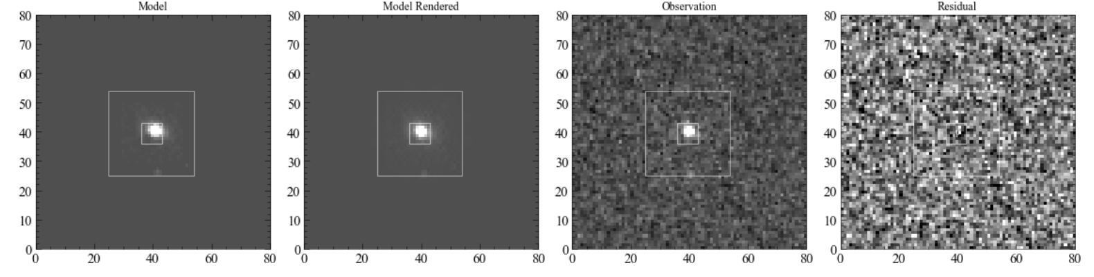
Some hypothesis:
- pointing (I don't think that will cause this wrong behavior)
- conversion from flux to magnitude (but the flux value is very large, ~1700, even for the star object)
- My flux is not normalized before modeling (theirs fluxes are all smaller than 1). And They used some way to scale to back after the modeling. Does Roman has the same thing?
- My data has too little bands? - I can either send more data inside, or shut down some of their bands to see how it behaves.
- They also have that 1.8 factor in front of the flux of galaxy. Maybe that's what I'm missing? But that is before the fitting... Why they have this 1.8 factor?
Learn about the simulation process for this lightcurve? How do they deal with fluxes? Here:
arxiv.org/pdf/2204.13553
Compare from difference image method? From paper (maybe Lauren) or from my method, to see what's the flux value extracted.
What exactly is the flux extracted? Is it integrated flux over the supernovae pixel region, or it's just the psf?
Examine the flux extracted for the star.
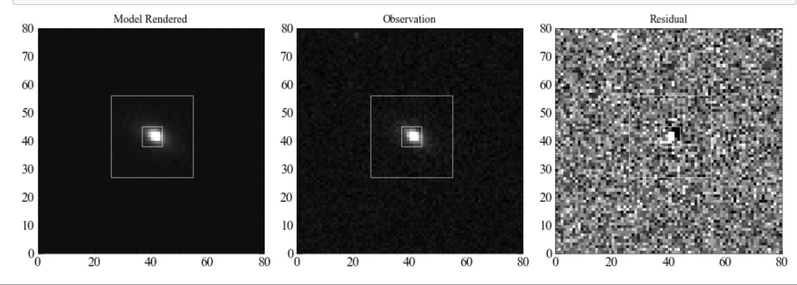
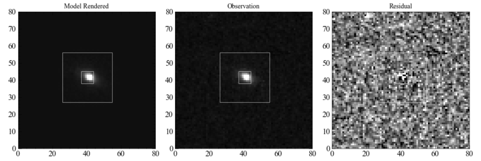
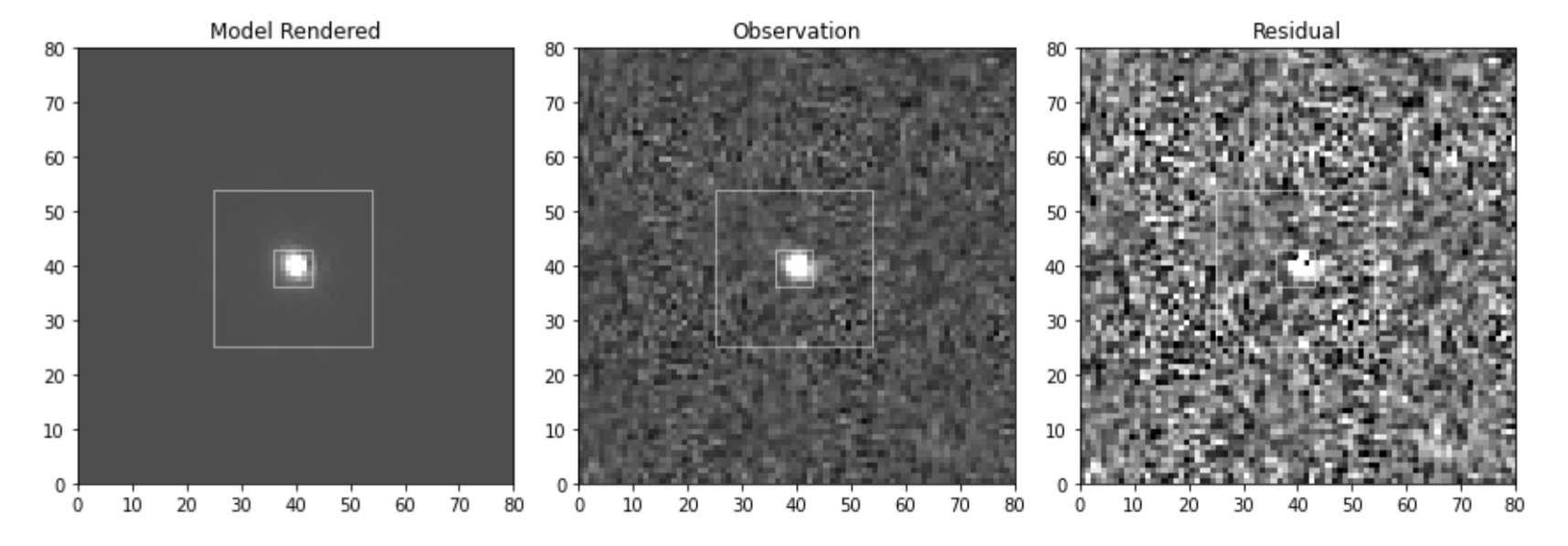
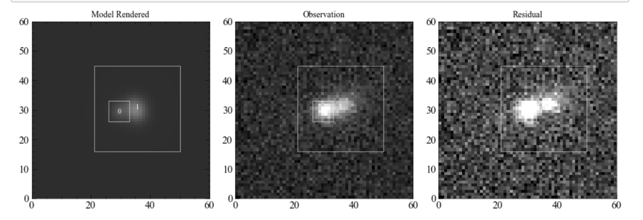
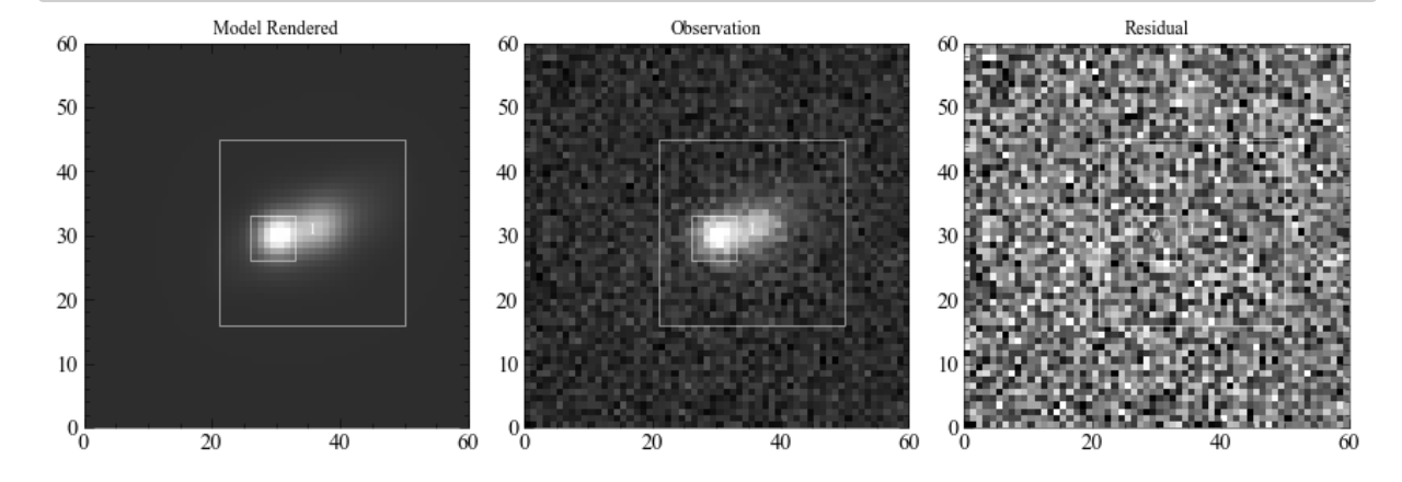
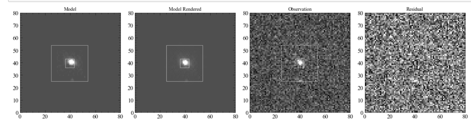
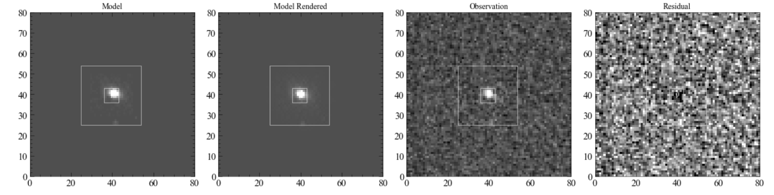
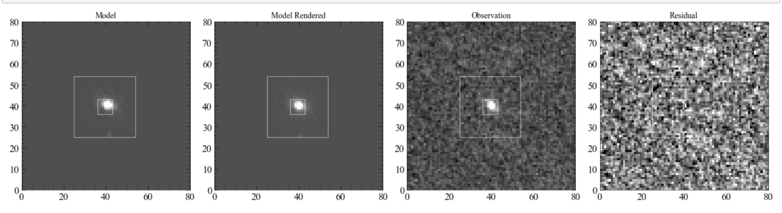
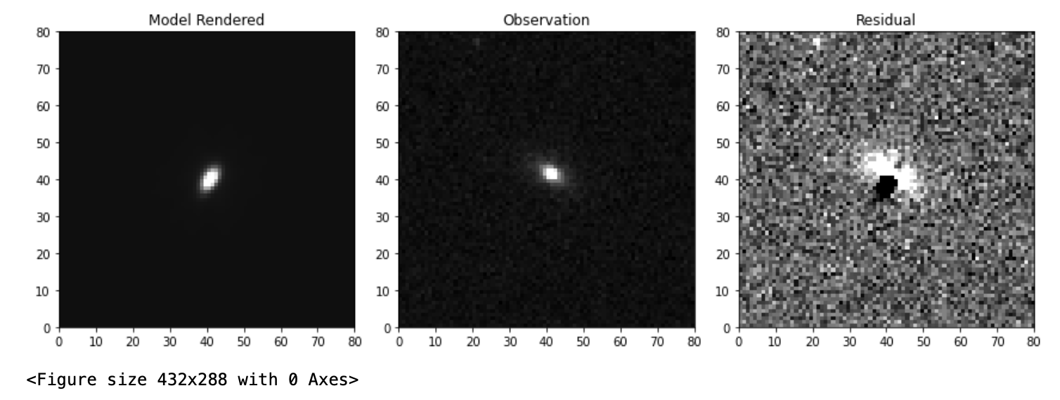
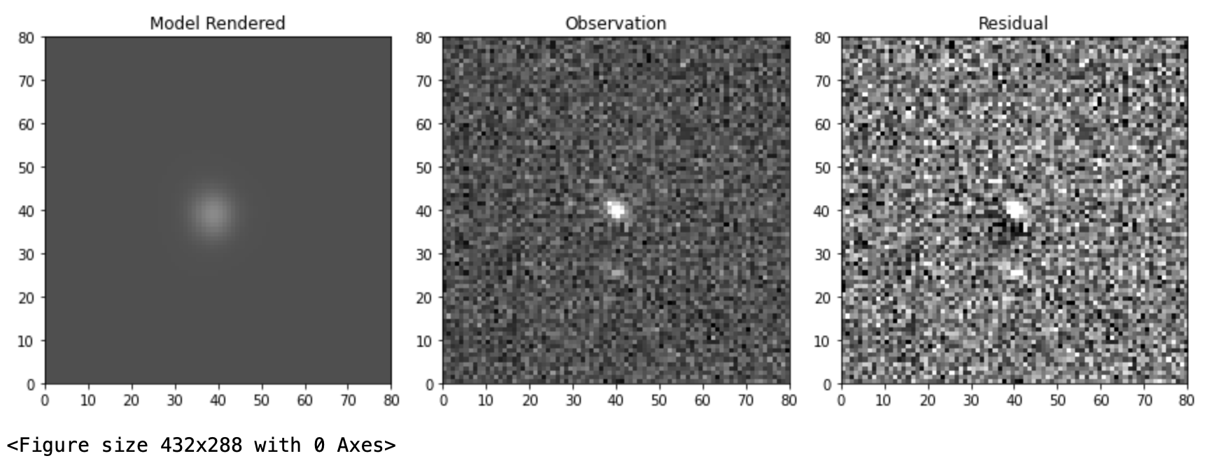
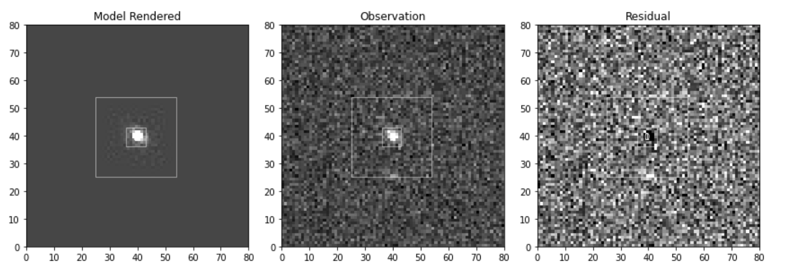
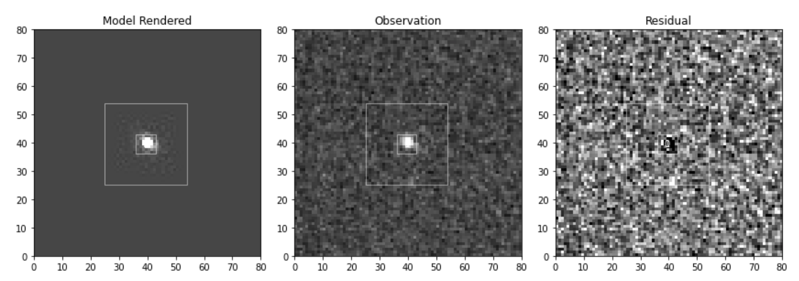
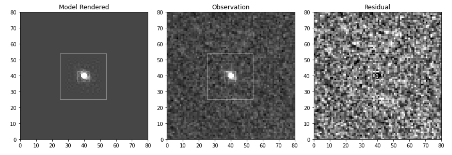
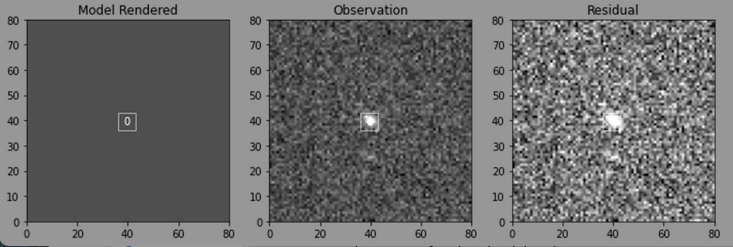
Does the image set (model, observation, residual) share the same scale?
Yes. They all get passed the same norm argument in the scarlet2.plot.scene function. for rendered and observed, but residual has a different scale.
How to analyse the residual statistics?
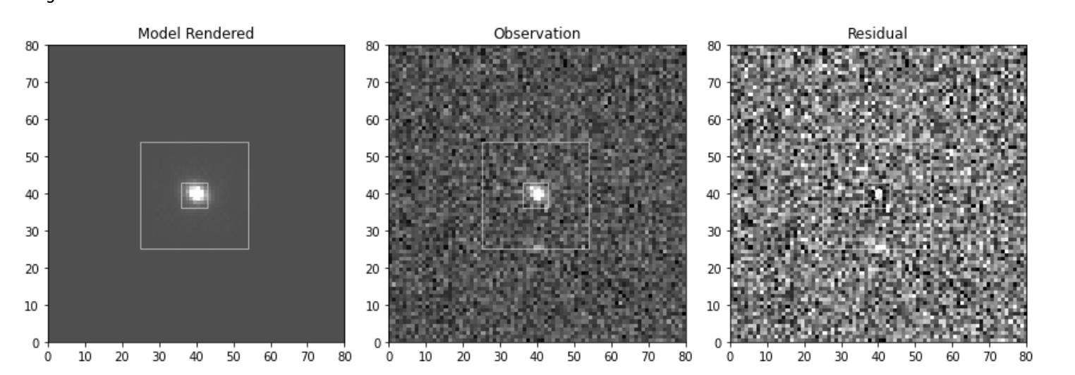
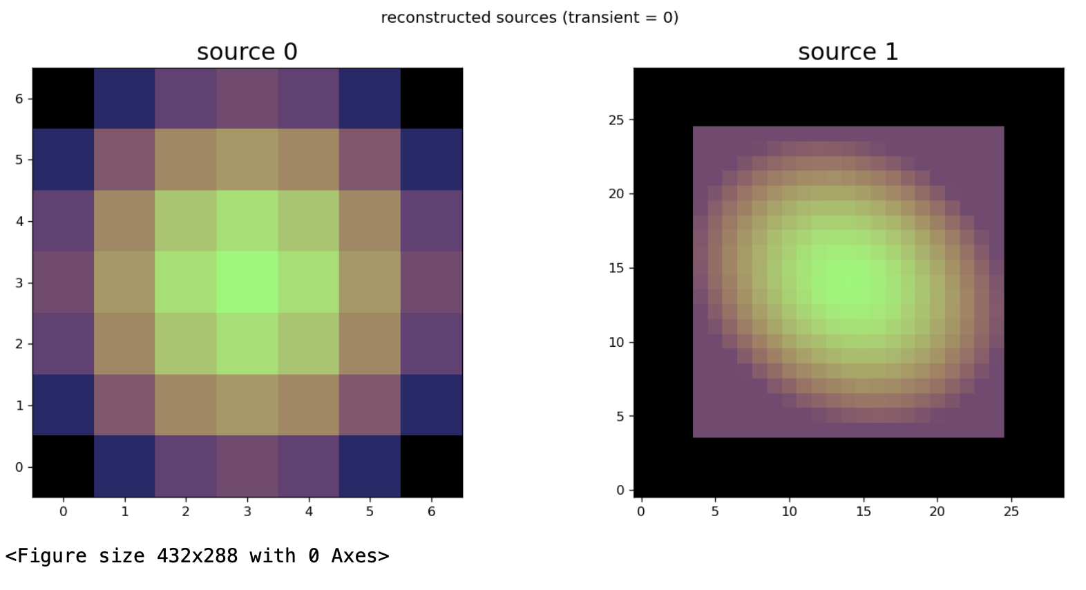
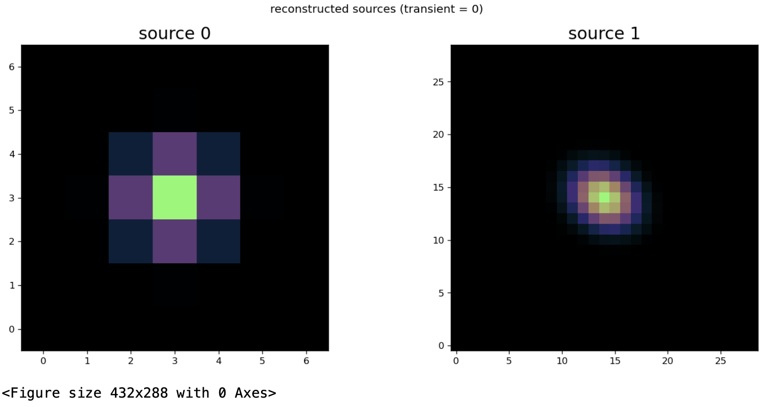
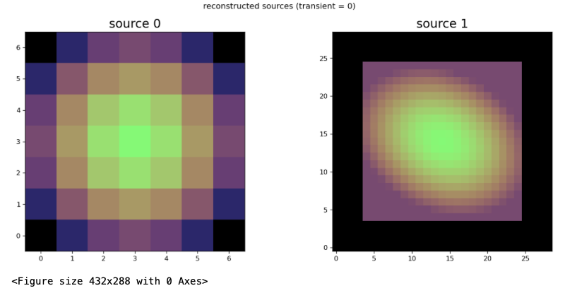
to get the rendered model:
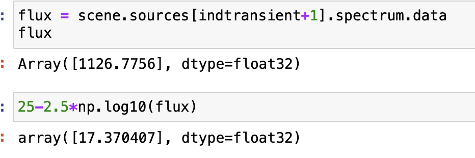
model_test = scene.sources[1]() # 1 is the index for the constant star/galaxy
rendered = observations_sc2[0].render(model_test)
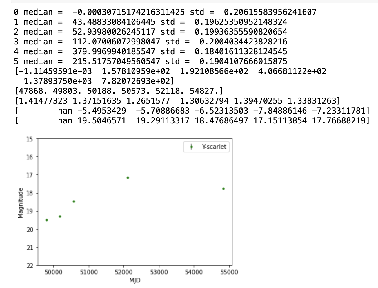
for star:
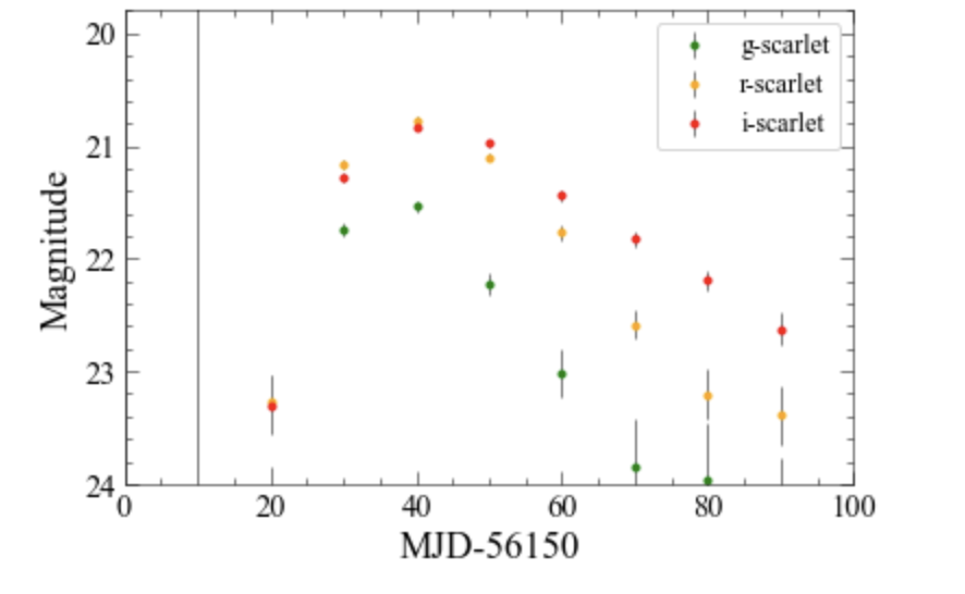
flux after fitting: 1126.7756, mag=17.37
12-29
Todo:
Check aligned images
understand code to construct model
Double subtracted background: img preprocessing and during segmentation process. Fixed this, but result looks the same.
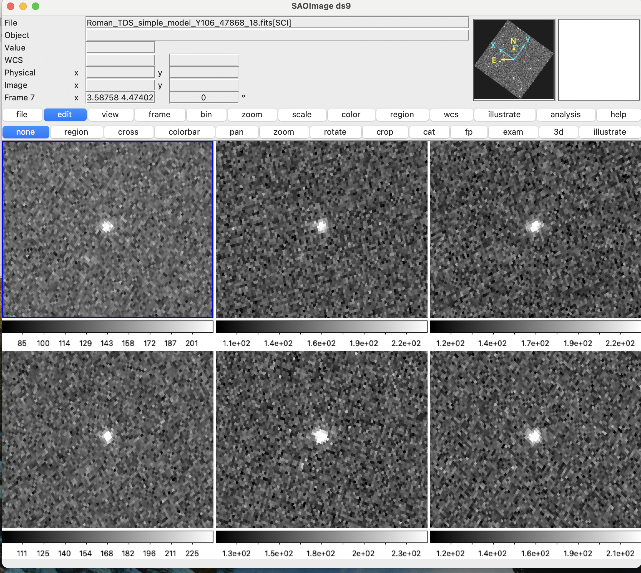
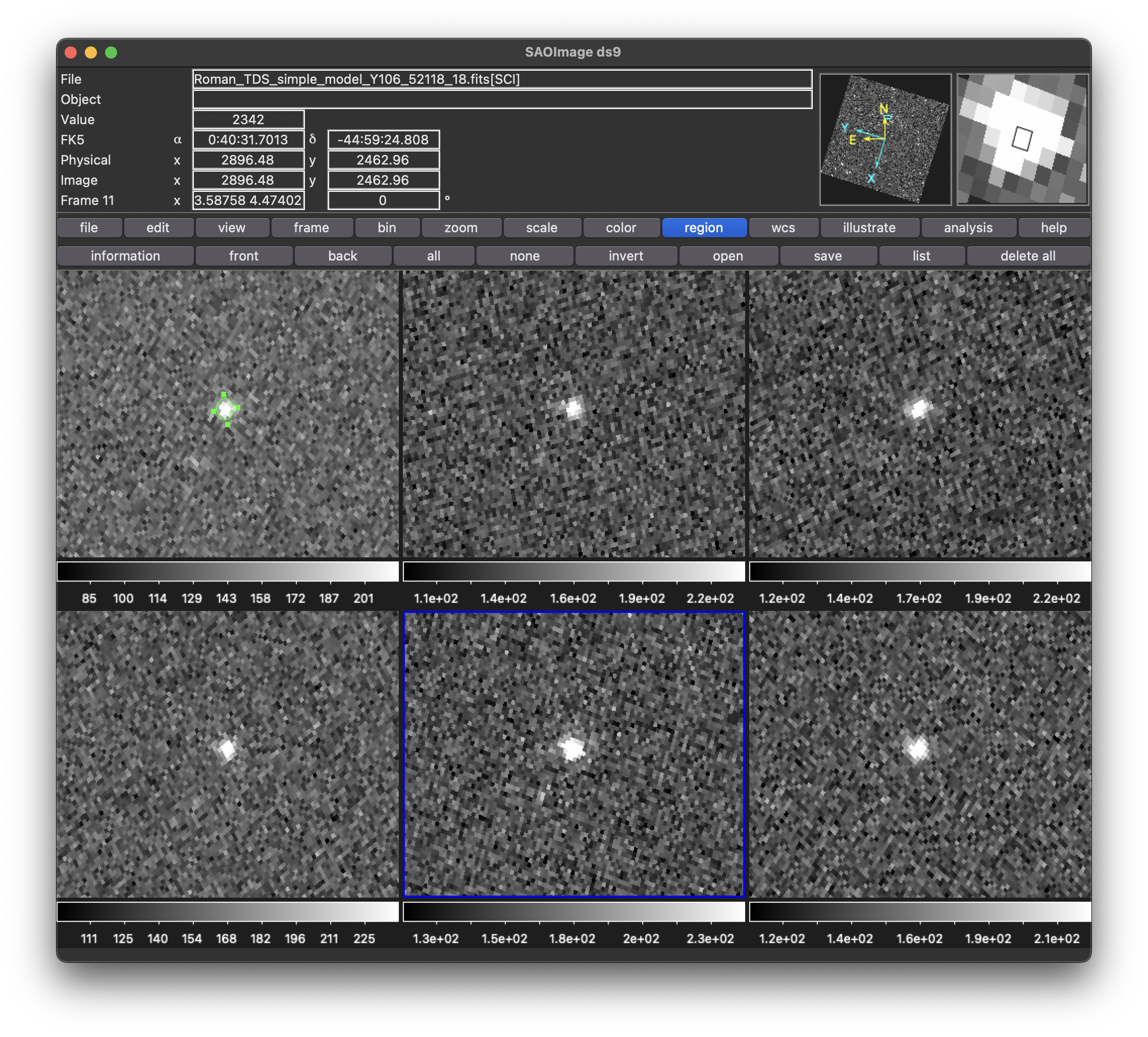
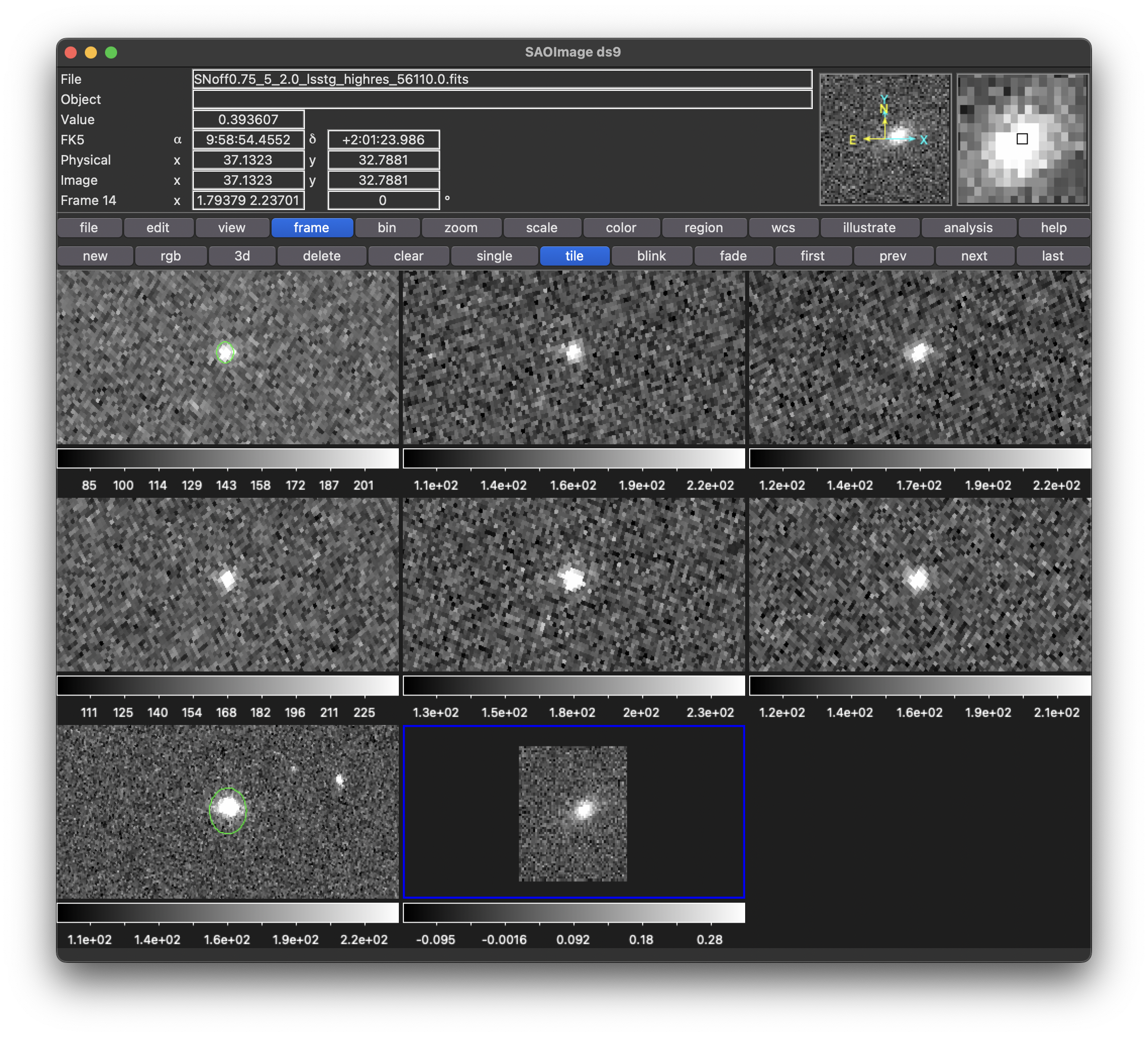
Plotted from DS9:
tried to through wcs to scarlet object, without reprojecting previously. It won't work.
Tried to shut down the spectrum parameter: looks same and seems like the last part need spectrum?
After fit:
In the paper it says to model the spectrum of the galaxy, plus the flux of SN, plus their positions, is it saying that the "spectrum:0" is actually flux of the supernova?
Answer: spectrum is actually their flux! (maybe because now I only have one band.)
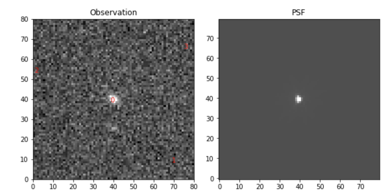
Re-run including the spectrum parameter. Now it detects 4 sources???
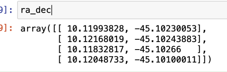
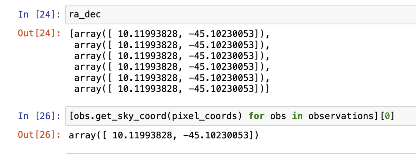
Multiple RA and Dec for source detection
But rerun the cell that do the source detection, it works. Not sure why...
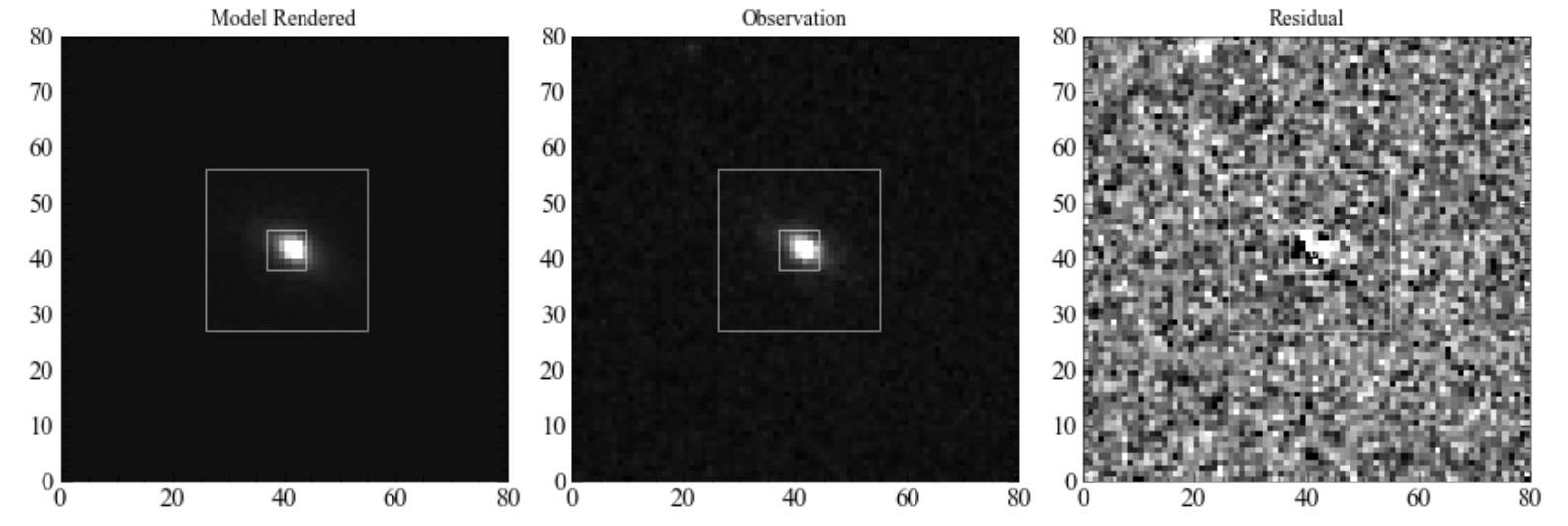
Now try to run Charlotte's code, so far it looks very different. But the fitting looks great actually? Why the first observation is not the same?
Before fit:
After fit:
It takes hours to fit....
Next possible steps: see how this works, if it's not working, maybe consider using the older version of scarlet2 to try to regenerate all the plots?---- AHHHHHH it works!!!!
If it works, then try to directly migrate my previous Roman pre-processing to this code.
If still doesn't work, maybe add more images so that it has spectrums? Or take off the spectrum paramter while fitting?
Notes on paper:
I made Charlotte's code work!!!!!
From my code:
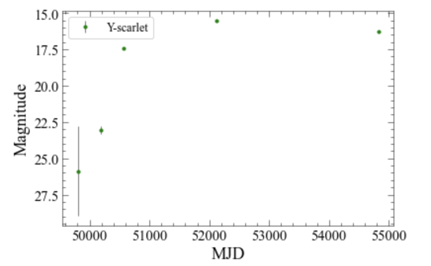
Magnitude:
From Hers:
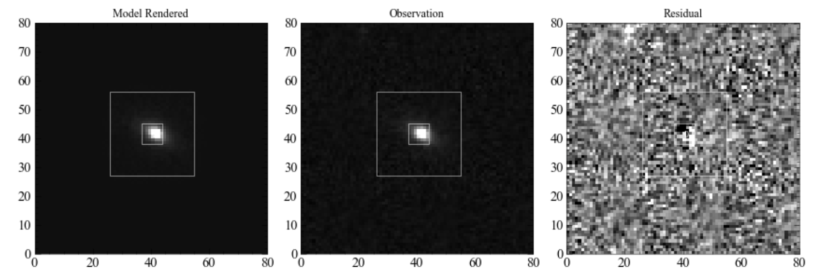
I now migrate all the data pre-processing steps to this worked code (which reproduced Charlotte's result)
For each image: from img 0(galaxy) to img 5
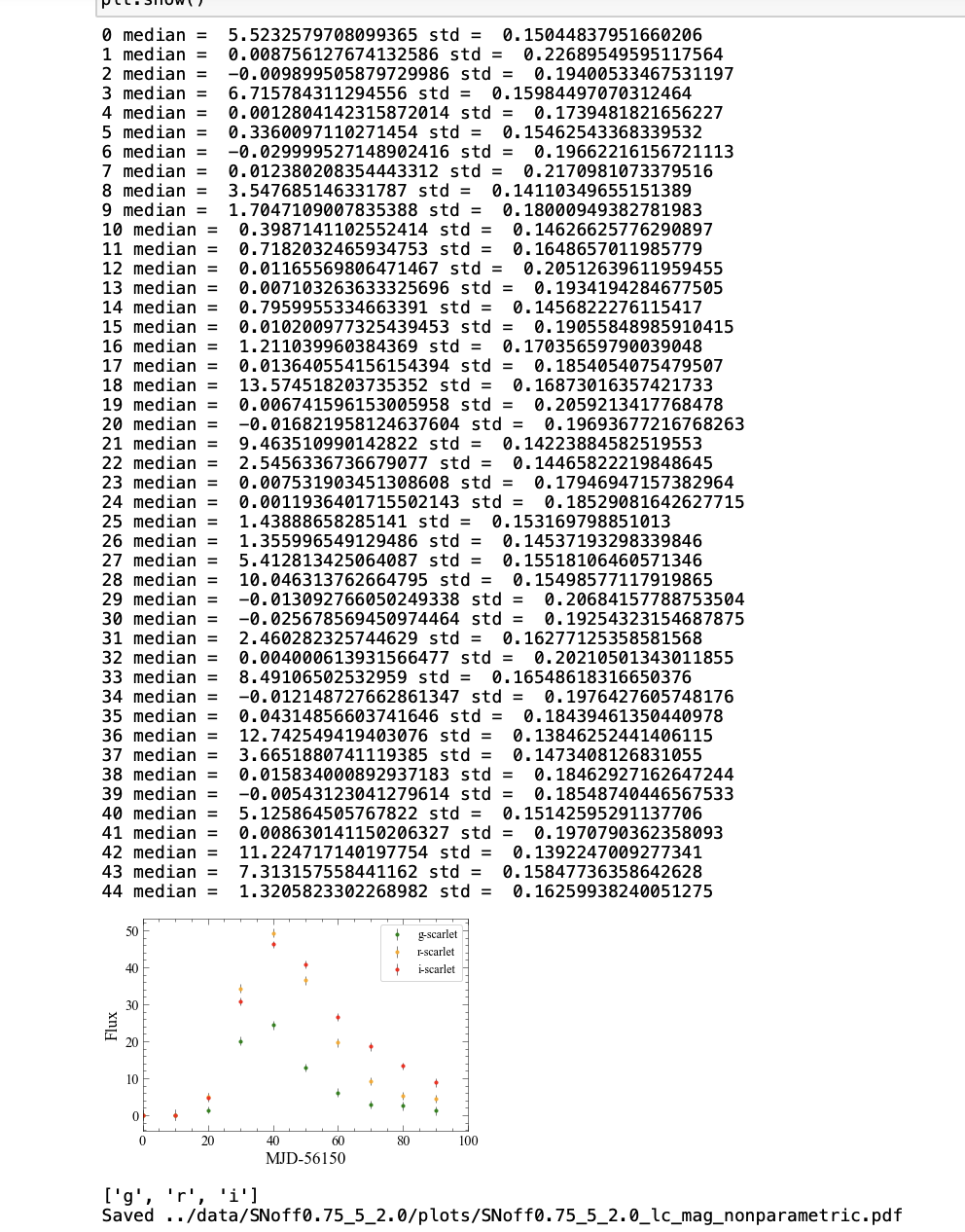
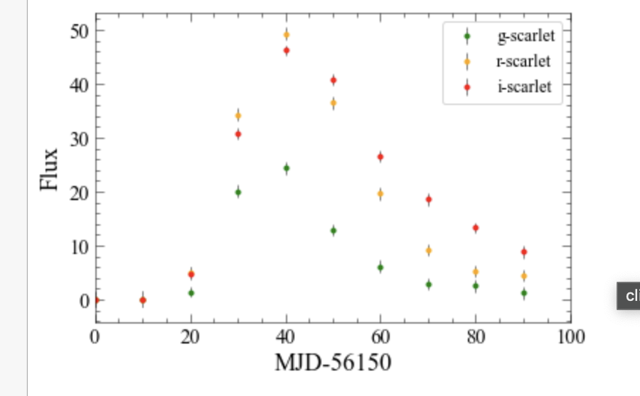
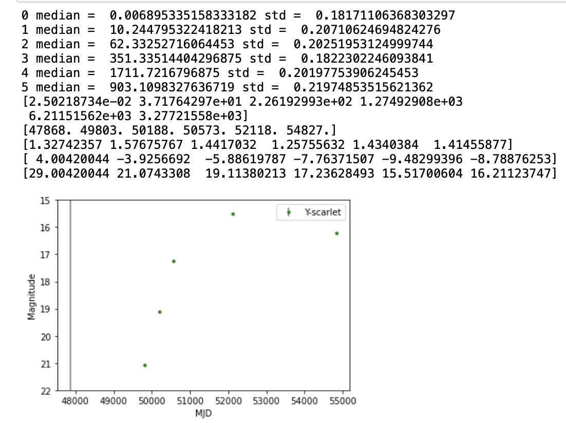
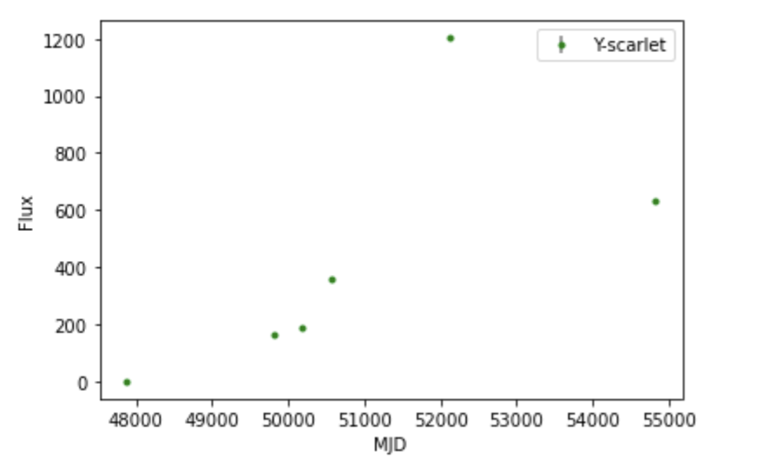
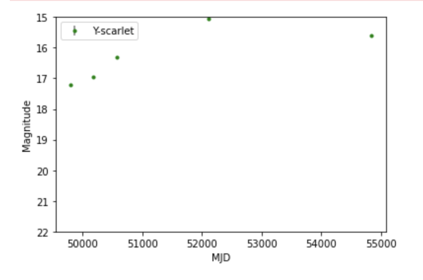
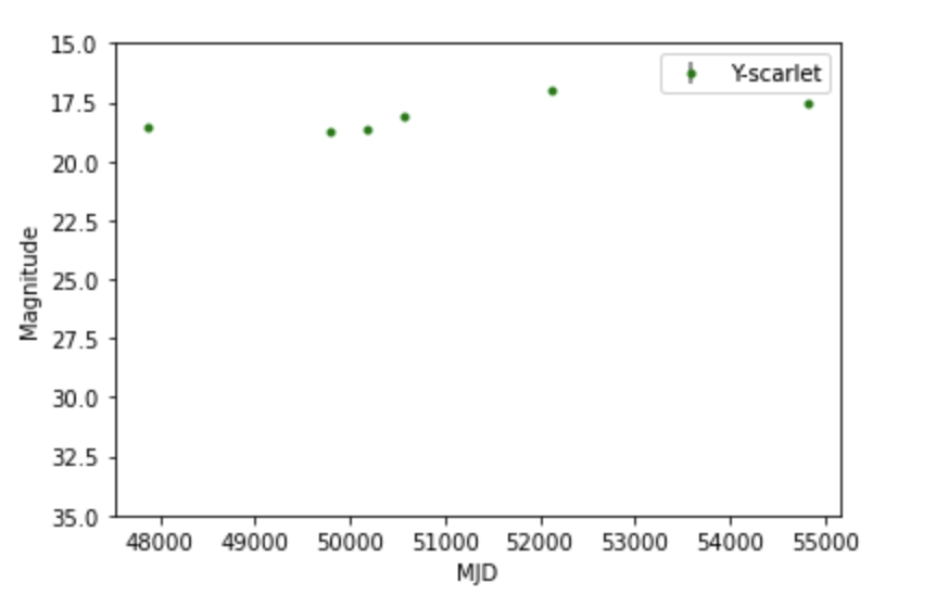
Light curve:
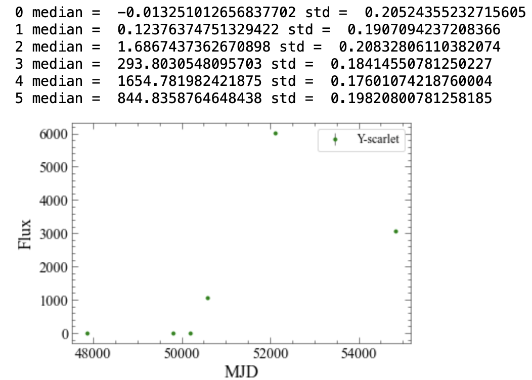
From DS9, the last 2 images do look very bright for the central pixels... 2000 something for the central pixel.
The forth:
The fifth:

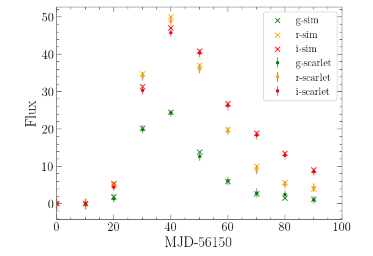
Some new finding!!!Their flux seems to be normalized.
12-28
Scarlet: revising psf and if not working, do it for the fixed star
#notes
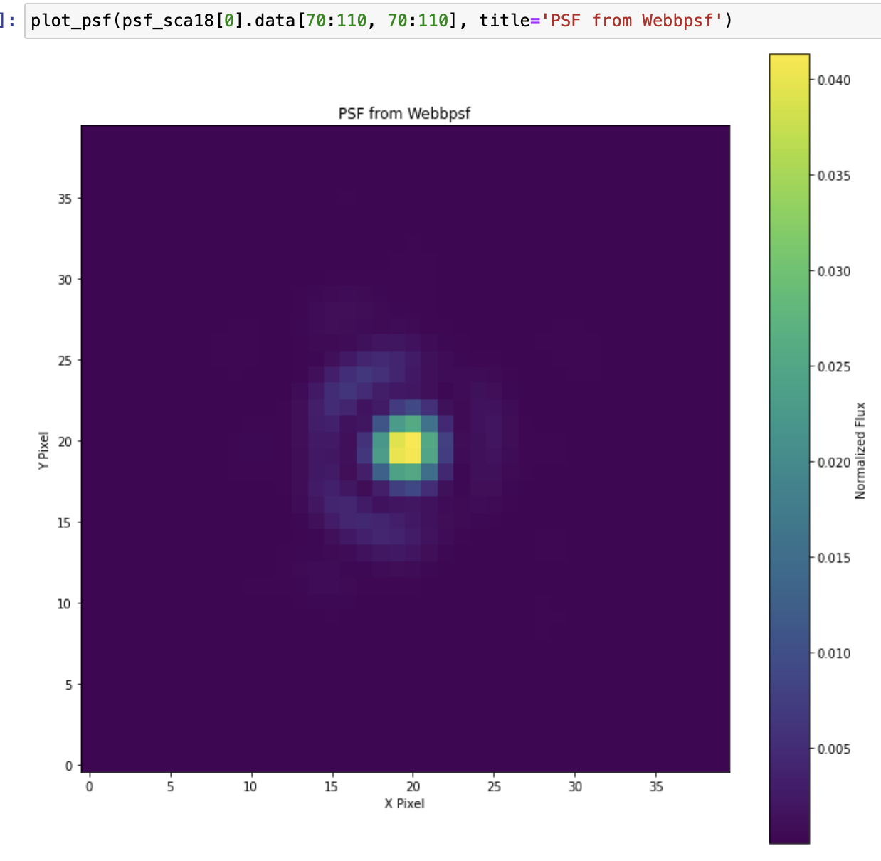
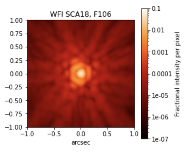
psf_sca18 = wfi.calc_psf() returns a hdulist. It has header, and data.
From Webbpsf, it looks similar to what I got from Galsim, the asymmetry:
Current scales:
-
psf_sca18[0].header['PIXELSCL']
Value: 0.0275 -
with cd matrix:
cd11 = hdu_ref[0].header['CD1_1']
cd12 = hdu_ref[0].header['CD1_2']
cd21 = hdu_ref[0].header['CD2_1']
cd22 = hdu_ref[0].header['CD2_2']
scale = 3600. * np.sqrt ((cd112+cd212+cd122+cd222)/2.)
Value: 0.10583060241974003 -
with wcs:
wcs_ref.pixel_scale_matrix.diagonal().mean() * u.deg.to(u.arcsec)
Image Pixel Scale: 0.08397533045026008 arcsec/pixel
Now using: proj_plane_pixel_scales method below:
Note for calculating pixel_scales:
Method 1: Using proj_plane_pixel_scales
from astropy.wcs.utils import proj_plane_pixel_scales

# Get pixel scales in degrees/pixel

pixel_scales_deg = proj_plane_pixel_scales(wcs)

# Convert to arcsec/pixel

pixel_scales_arcsec = pixel_scales_deg * 3600  # 1 degree = 3600 arcsec

print(f"Pixel Scales: {pixel_scales_arcsec} arcsec/pixel")
Method 2: Using pixel_scale_matrix
# Extract CD matrix
cd_matrix = wcs.pixel_scale_matrix

# Calculate pixel scale for each axis
import numpy as np

pixel_scale_x = np.sqrt(cd_matrix[0, 0]**2 + cd_matrix[0, 1]**2) * 3600  # arcsec/pixel
pixel_scale_y = np.sqrt(cd_matrix[1, 0]**2 + cd_matrix[1, 1]**2) * 3600  # arcsec/pixel

print(f"Pixel Scale X: {pixel_scale_x} arcsec/pixel")
print(f"Pixel Scale Y: {pixel_scale_y} arcsec/pixel")
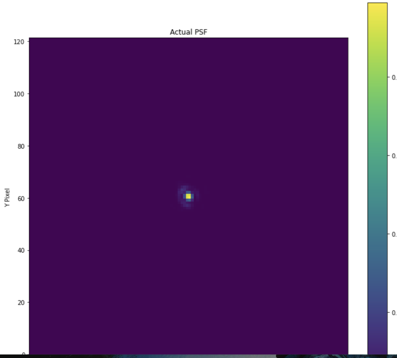
Now the question is: how to resample the psf images?
From Galsim?: Use interpolated image class and it works!!! Arbitrary Profiles — GalSim 2.5.3 documentation
Or from Webbpsf?
With resampled psf: new round of testing:
Somewhat better:

Alright...
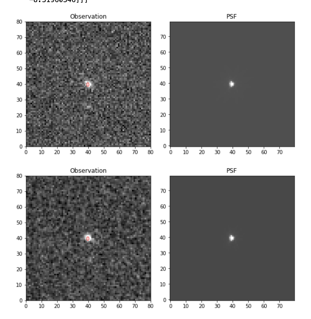
test on a star:
convert RA and Dec from Hours:Minutes:Seconds to decimal degrees:
0:40:35.6745,-45:00:34.397
->10.148635° , -45.009555°
Cutout shape is 80by80, to avoid extra sources in this region
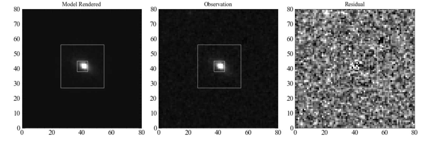
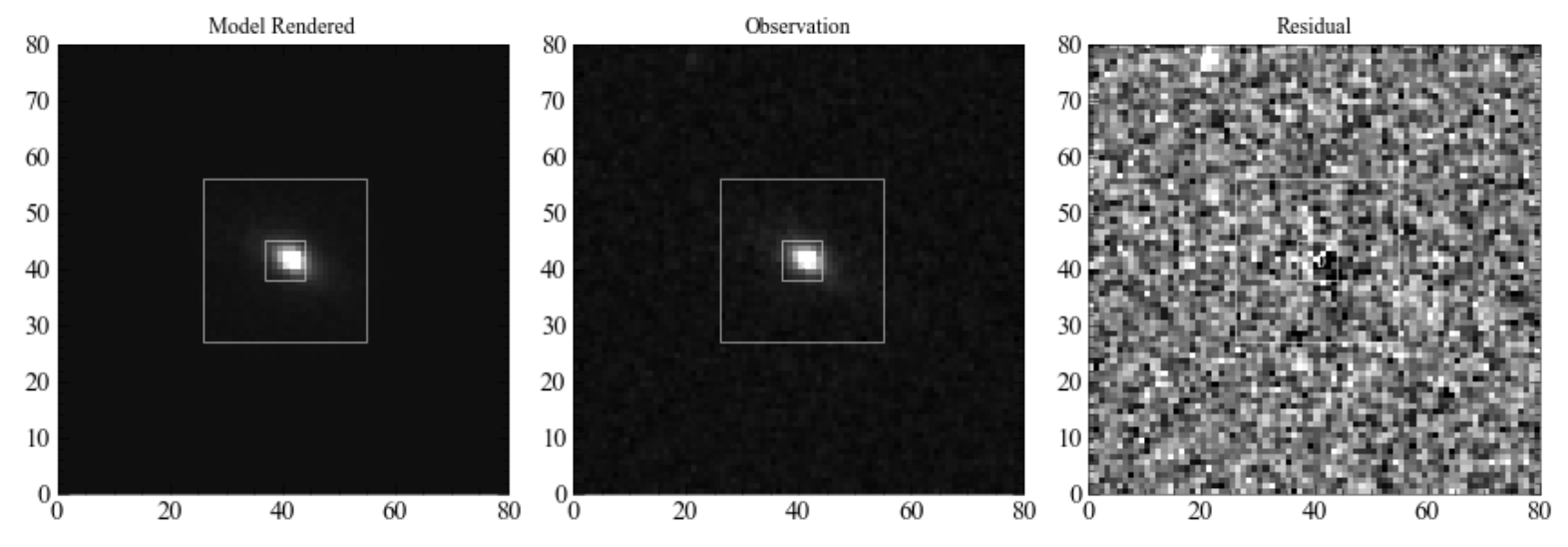
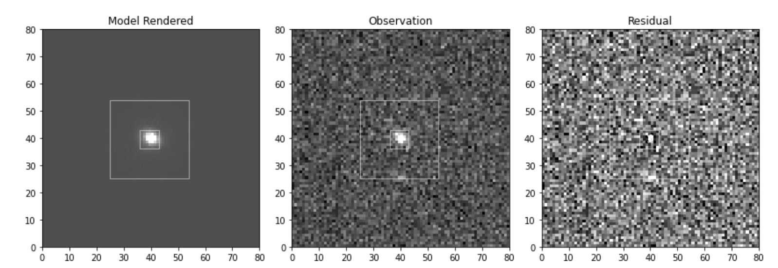
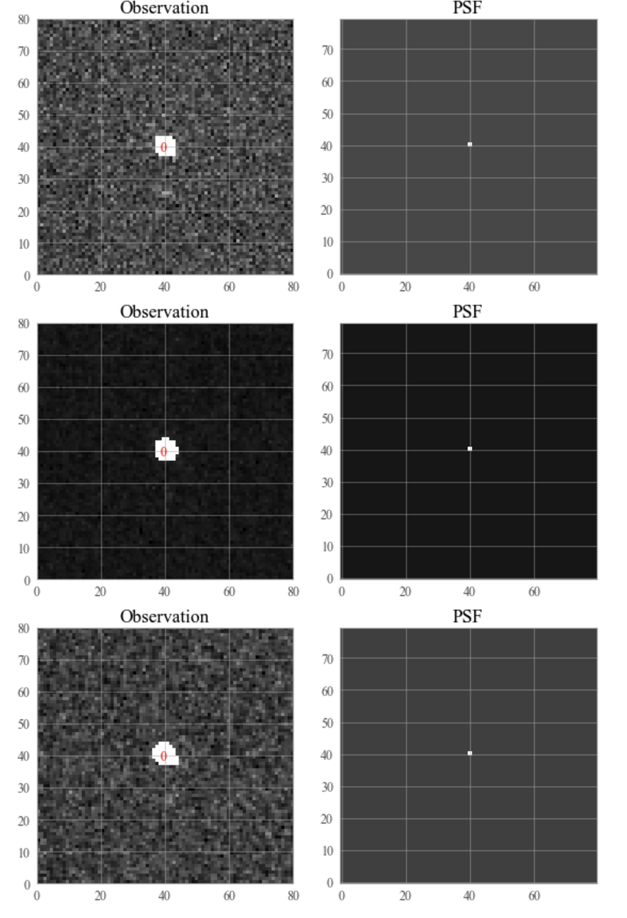
The rendered model looks like it's tilted... (shear in a wrong direction) for both this star object, and the previous SN+galaxy.
Next step: how they build model? Is that because there are two different sources? Run the whole thing with just galaxy model, and no SN source (re-write the model?)
MCMC process looks not changing anything (so probably it's not this part's issue)
Plot before the MCMC:
My rendered model also tilted in one direction...
Next: Make sure each image is aligned properly, check side by side if my construction of the model is correct.
Maybe try running Charlotte's code and see if it works?
Future: learn about the MCMC process.
12-27
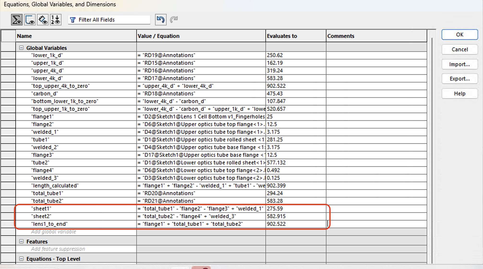
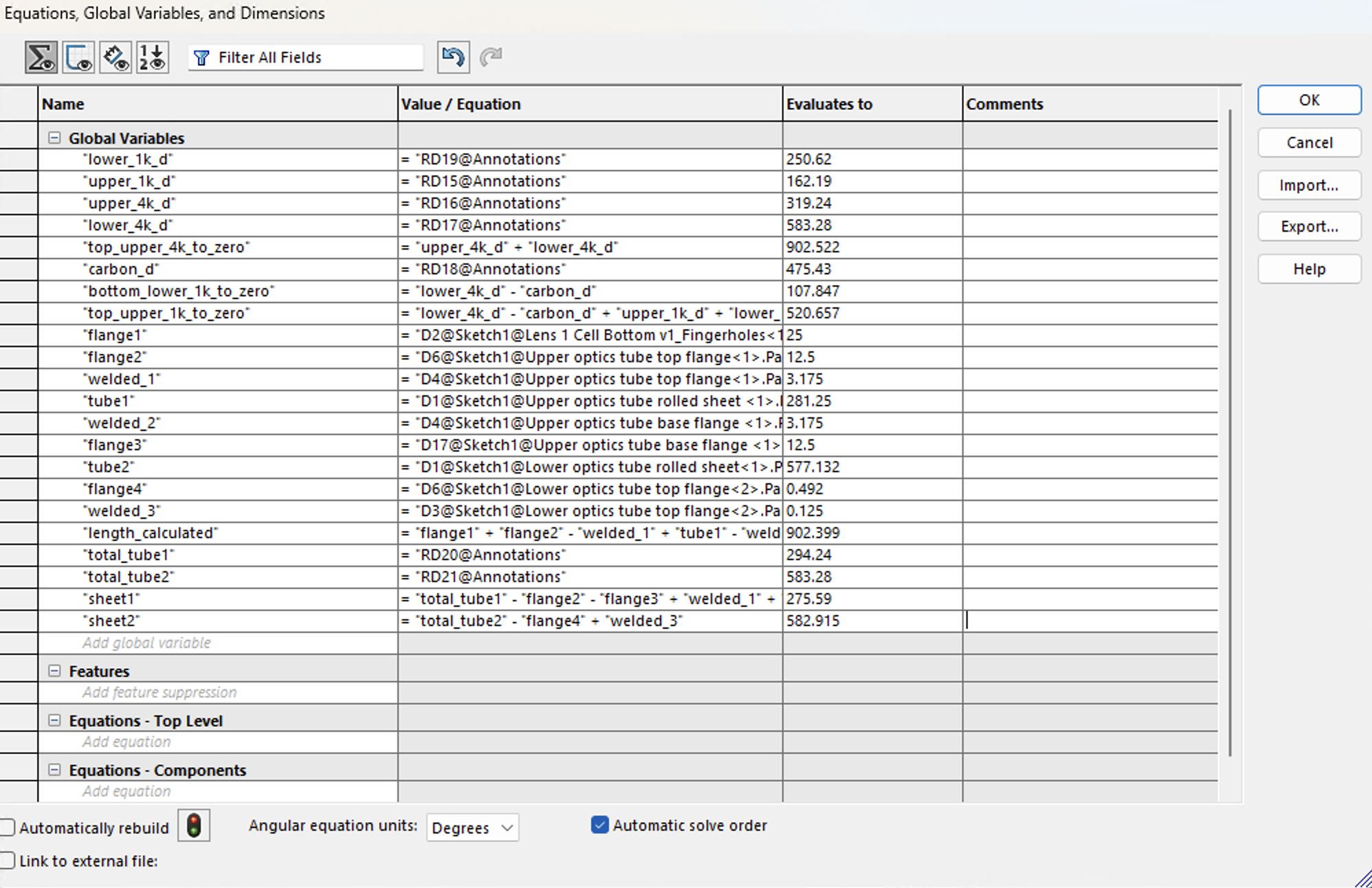
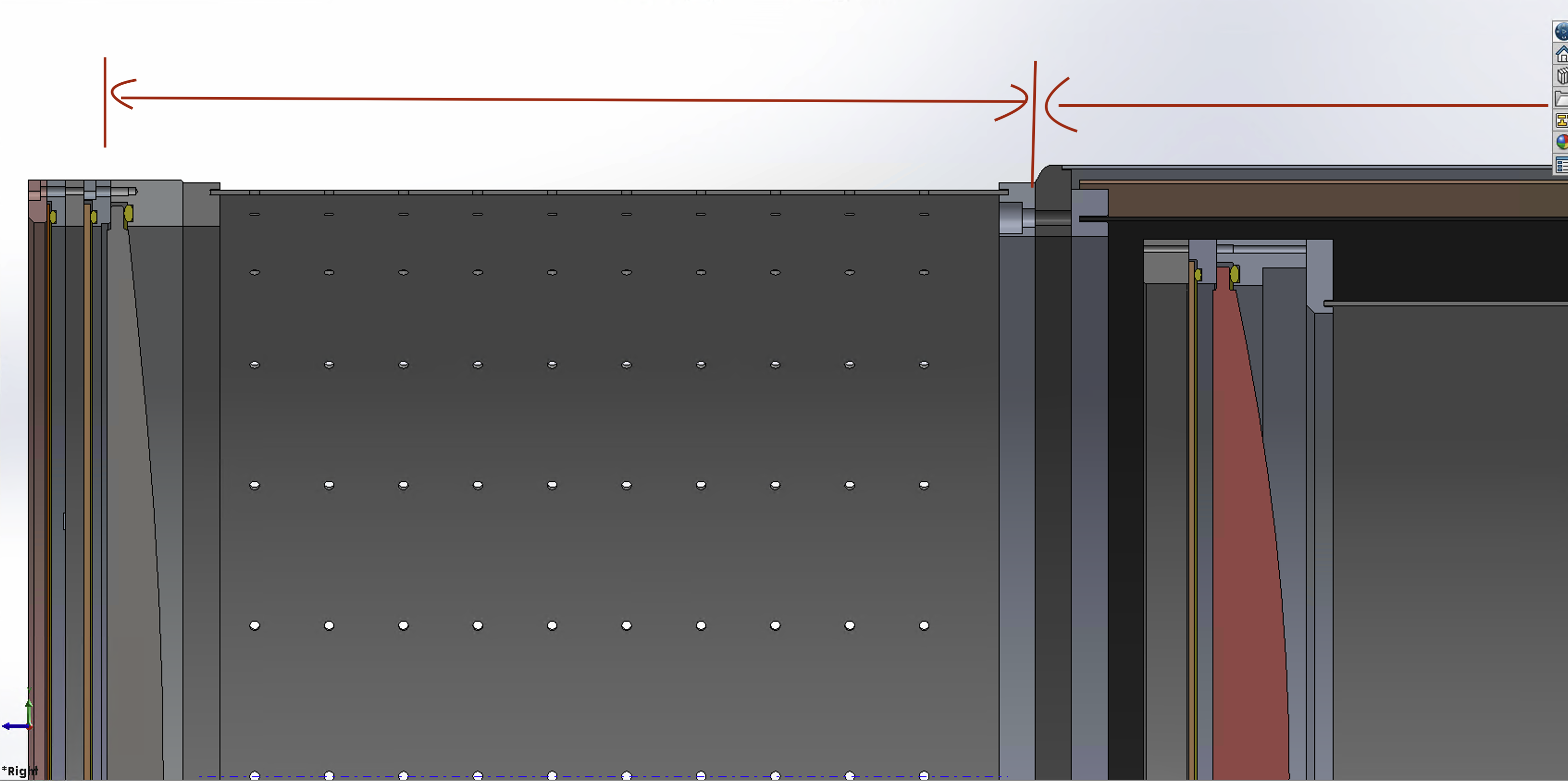
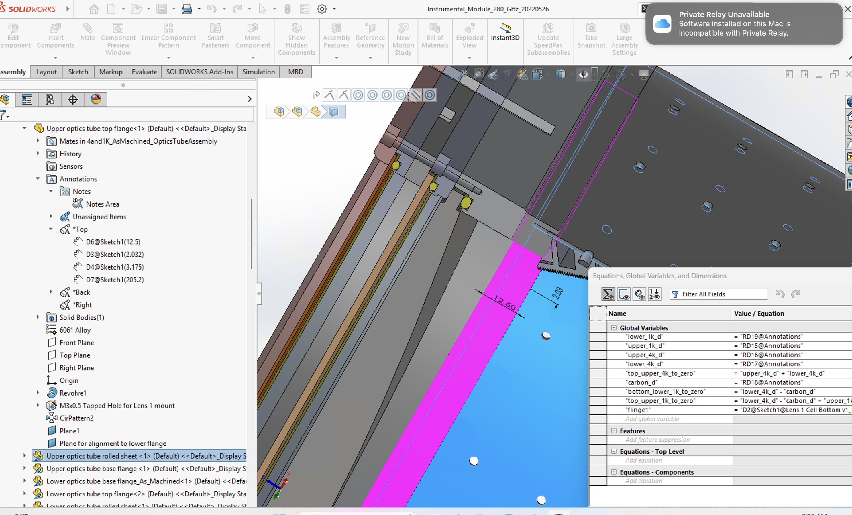
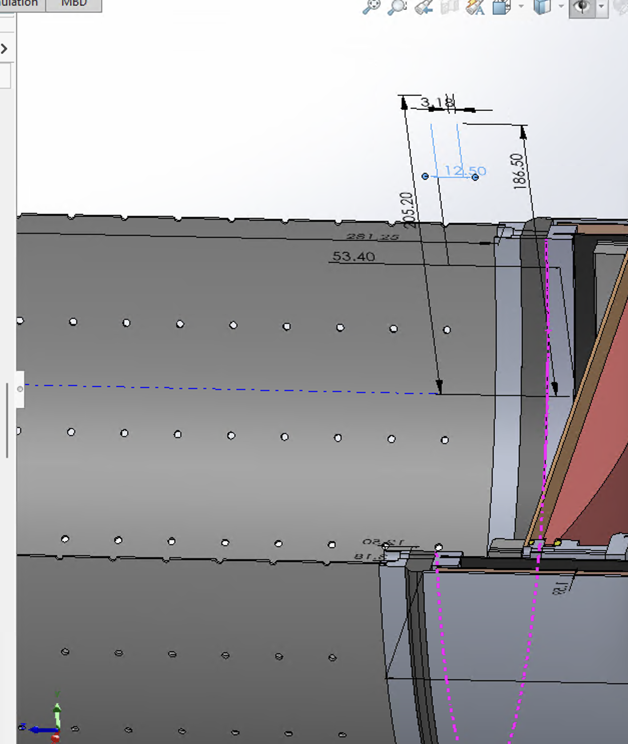
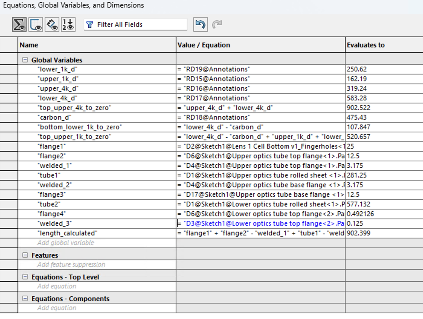
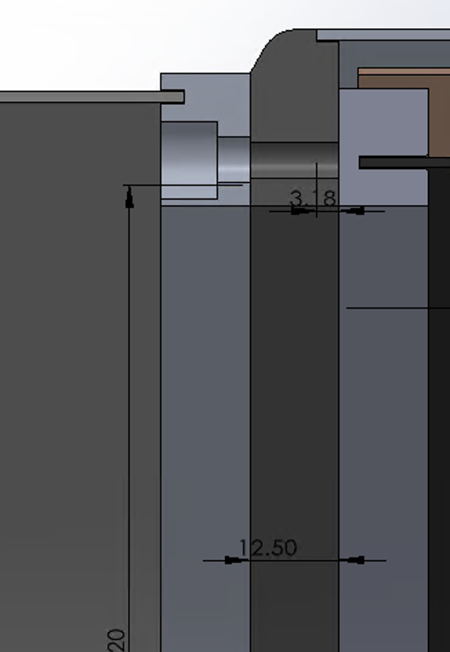
Parametrization:
From Ben:
the lengths of the rolled sheets should change in response to the change in the overall length of each part. The total distance from the 4K flange to lens 1 should change in response to the change in the sum of overall distance changes
Scarlet:
Revising PSF
pixel scales: CD matrix from WCS of the fits file.
WCS: standard transformation from pixel coordinates to real-world coordinate
CD matrix: the linear transformation from pixel coordiante to real-world coordinate:
x_0, y_0: Reference pixel coordinates (CRPIX1, CRPIX2).
CDELT and PC Matrix Representation:
Difference between CD matrix and Jacobian of PSF in galsim profile building:
how to build Roman PSF:
Troxel's paper:
arxiv.org/pdf/1912.09481
GitHub - matroxel/roman_imsim at 74a9053653bdafb04ffb51dff2500e5f82632c85
Documentation: Point Spread Function Modeling — romanisim 0.7.1.dev3+gec38b29.d20241216 documentation
Webbpsf: Roman Instrument Model Details — webbpsf vdev
Galsim.Roman package: The Roman Space Telescope Module — GalSim 2.5.3 documentation
Try to use Webbpsf to build Roman PSF
-
Install Webbpsf: need to download data from the website, and add an environment parameter
-
A useful jupyter notebook: Jupyter Notebook Viewer
-
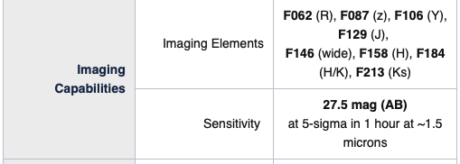
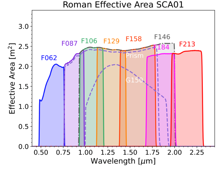
Try to use Webbpsf, but it does not have Y106 band? But from this document it should have?stsci.edu/files/live/sites/www/files/home/roman/_documents/AAS229-WebbPSF-Long.pdf Also from this: stsci.edu/files/live/sites/www/files/home/roman/_documents/roman-mission-operations-tools.pdf
-
Y106 is the same as F106.... Nobody states this directly.... But I think this is the proof: WFI Quick Reference - Roman User Documentation
-
-
Filter information: Wide Field Instrument - Technical - Roman Space Telescope/NASA
-
-
Followed this document to generate a psf using Webbpsf: Roman Instrument Model Details — webbpsf vdev
-
-
Understanding detector_position parameter in wfi module. Why and how to set it?
- SCA: each SCA is a large CCD or CMOS sensor, with 4096 x 4096 grid
- detector_position: A tuple representing the (x, y) pixel coordinates within a specific SCA where the PSF is calculated.
- PSF is position dependent.
- This is Monochromatic PSF: The PSF is calculated assuming light at a single wavelength.
The WFI is not a separate telescope but the primary instrument aboard Roman.
WFIRST stands for Wide Field Infrared Survey Telescope. It was the original name of what is now known as the Nancy Grace Roman Space Telescope.
12-26
Shrink the size of PSF from galsim roman:
The full pupil plane images are 4096 x 4096, which use a lot of memory and are somewhat slow to use, so we normally bin them by a factor of 4 (resulting in 1024 x 1024 images).
Shrink from bin=8 to bin=64, so that the psf data shape size is smaller than the cutout data shape.
- Working code:
roman_filters = roman.getBandpasses(AB_zeropoint=True)
star = galsim.DeltaFunction()
bandpass = roman_filters['Y106']
star = star * galsim.SED(lambda x:1, 'nm', 'flambda').withFlux(1., bandpass)
psf = galsim.roman.getPSF(15, 'Y106', n_waves=10, pupil_bin=64) # pupil bin size
psf_img = galsim.Convolve(star , psf)
psf_im = psf_img.drawImage(bandpass=bandpass)
changed psf from
Check on the psf: it looks weird: it has this little antisymmetric ring thing
From Troxel's paper: You will have such ring thing, but it's symmetric? How do they produce it?
A synthetic Roman Space Telescope High-Latitude Imaging Survey: simulation suite and the impact of wavefront errors on weak gravitational lensing - ADS
After the convolution of PSF with source object (star): the drawImage method:
Figure out the meaning of scale:
The GSObject base class — GalSim 2.5.3 documentation
drawImage(image=None, nx=None, ny=None, bounds=None, scale=None, wcs=None, dtype=None, method='auto', area=1.0, exptime=1.0, gain=1.0, add_to_image=False, center=None, use_true_center=True, offset=None, n_photons=0.0, rng=None, max_extra_noise=0.0, poisson_flux=None, sensor=None, photon_ops=None, n_subsample=3, maxN=None, save_photons=False, bandpass=None, setup_only=False, surface_ops=None)
Find a star like object to do the same process and see if it's also too dim.
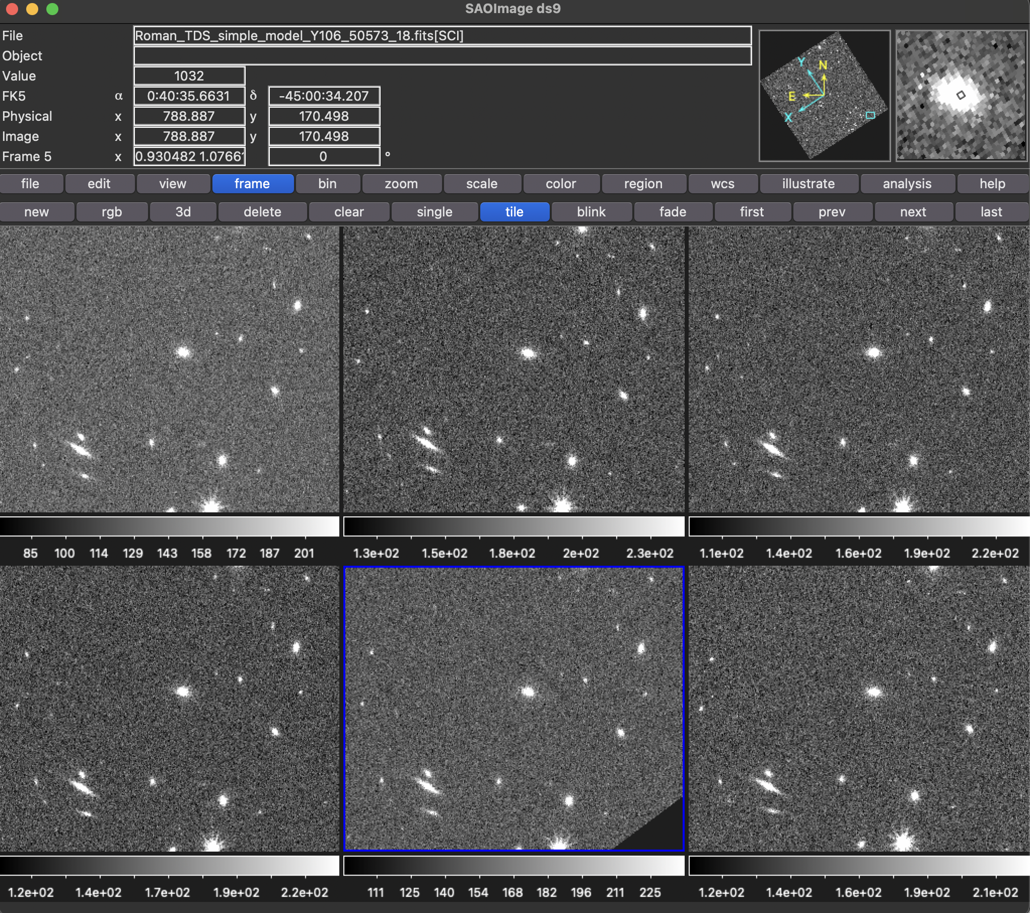
DS9 align images:
frame(in the middle)-> tile-> new
file, open fits file
frame (upper menu) ->match-> wcs
Steps can be found from this documentation of DS9:
Using SAOImage ds9 - CIAO 4.17
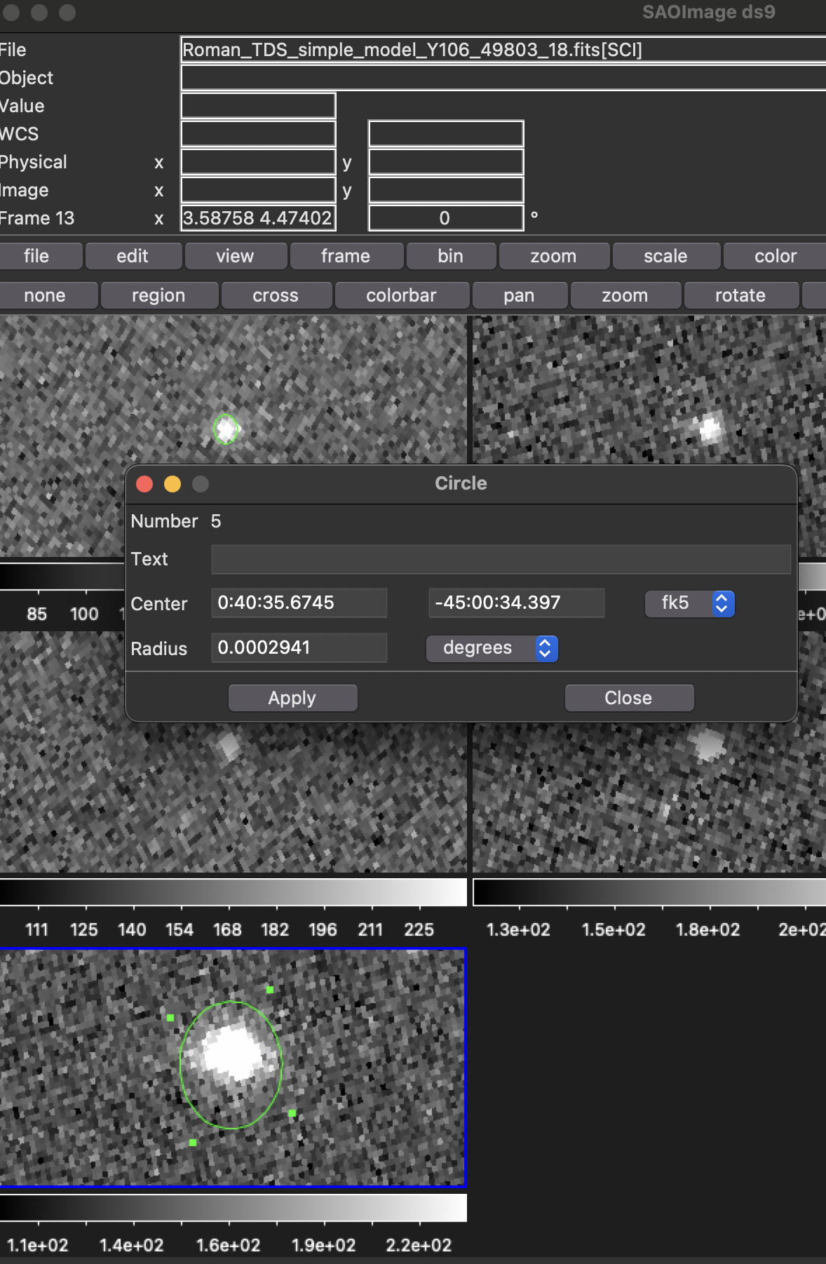
Use this as test:
0:40:35.6745,-45:00:34.397
convert to decimal, and then run the whole thing.
Tips: fast way to navigate with a RA/DEC, choose region, double click to start a new region, and then type the location, and radius, to mark a circular region. Like this:
12-25
Scarlet2:
Change previous psf placeholder to Roman psf
Operate the whole process with a constant start?
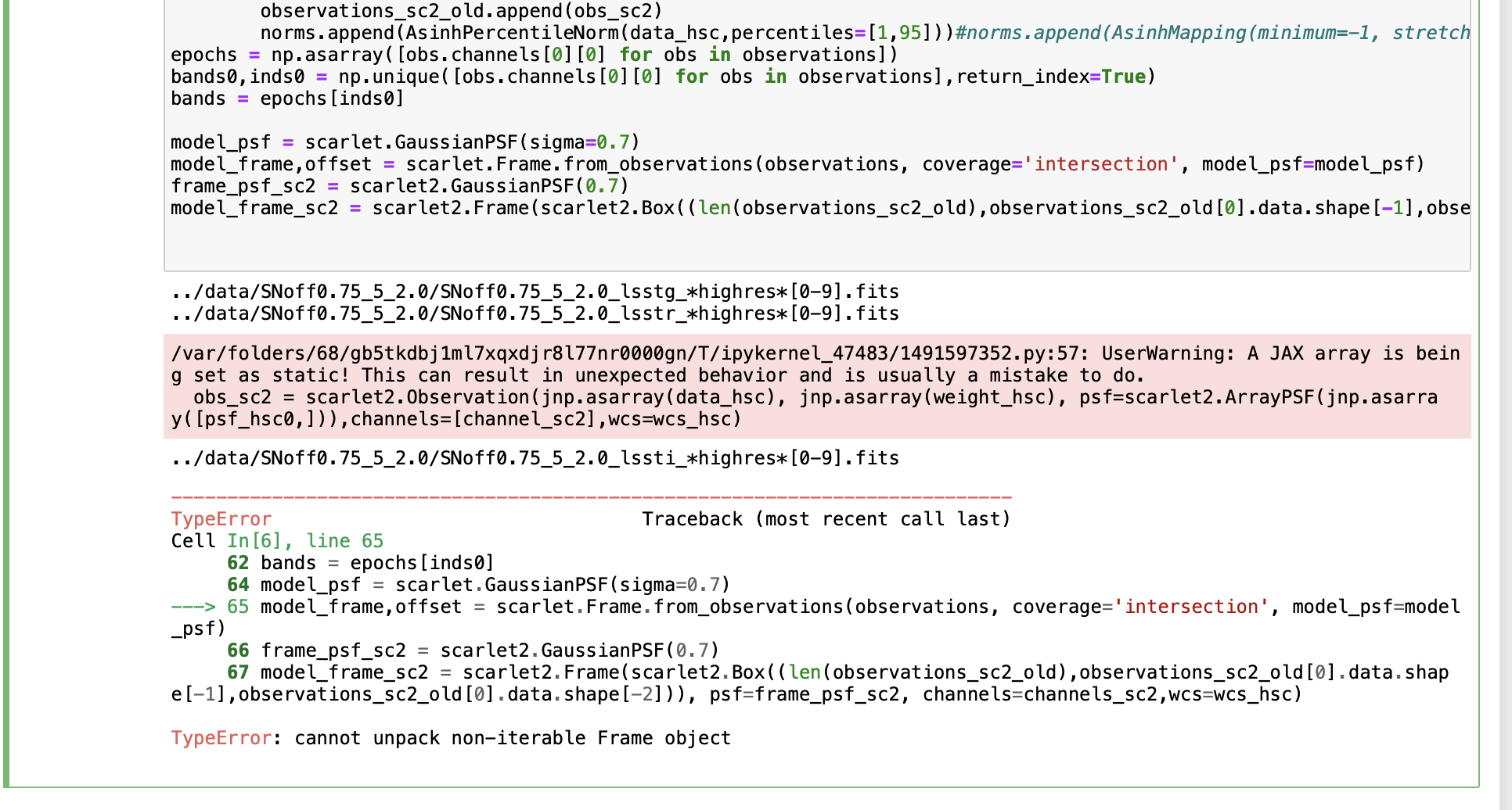
Error with the matching scarlet2 and scarlet frame:
---------------------------------------------------------------------------
ValueError                                Traceback (most recent call last)
Cell In[30], line 40
     38 # Align observations to model frame for scarlet2
     39 for obs in observations_sc2:
---> 40     obs.match(model_frame_scarlet2)

    [... skipping hidden 1 frame]

File ~/Documents/2_Research.nosync/RomanScarlet2/scarlet2/observation.py:93, in Observation.match(self, frame, renderer)
     90         renderers.append(PostprocessMultiresRenderer(frame, self.frame))
     92     else:
---> 93         renderers.append(ConvolutionRenderer(frame, self.frame))
     95 if len(renderers) == 0:
     96     renderer = NoRenderer()

    [... skipping hidden 3 frame]

File ~/Documents/2_Research.nosync/RomanScarlet2/scarlet2/renderer.py:83, in ConvolutionRenderer.__init__(self, model_frame, obs_frame)
     78 fft_shape = _get_fast_shape(
     79     model_frame.bbox.shape, psf_model.shape, padding=3, axes=(-2, -1)
     80 )
     82 # compute and store diff kernel in Fourier space
---> 83 diff_kernel_fft = deconvolve(
     84 obs_frame.psf(),
     85 psf_model,
     86 axes=(-2, -1),
     87 fft_shape=fft_shape,
     88 return_fft=True,
     89 )
     90 object.__setattr__(self, "_diff_kernel_fft", diff_kernel_fft)

File ~/Documents/2_Research.nosync/RomanScarlet2/scarlet2/fft.py:123, in deconvolve(image, kernel, padding, axes, fft_shape, return_fft)
    105 def deconvolve(image, kernel, padding=3, axes=None, fft_shape=None, return_fft=False):
    106     """Deconvolve image with a kernel
    107
    108     This is usually unstable. Treat with caution!
   (...)
    120         Axes that contain the spatial information for the PSFs.
    121     """
--> 123     return _kspace_op(
    124 image,
    125 kernel,
    126 operator.truediv,
    127 padding=padding,
    128 fft_shape=fft_shape,
    129 axes=axes,
    130 return_fft=return_fft,
    131 )

File ~/Documents/2_Research.nosync/RomanScarlet2/scarlet2/fft.py:159, in _kspace_op(image, kernel, f, padding, axes, fft_shape, return_fft)
    154         fft_shape = _get_fast_shape(
    155             image.shape, kernel.shape, padding=padding, axes=axes
    156         )
    157     kernel_fft = transform(kernel, fft_shape, axes=axes)
--> 159 image_fft = transform(image, fft_shape, axes=axes)
    160 image_fft_ = f(image_fft, kernel_fft)
    161 if return_fft:

File ~/Documents/2_Research.nosync/RomanScarlet2/scarlet2/fft.py:38, in transform(image, fft_shape, axes)
     33     msg = (
     34         "fft_shape self.axes must have the same number of dimensions, got {0}, {1}"
     35     )
     36     raise ValueError(msg.format(fft_shape, axes))
---> 38 image = _pad(image, fft_shape, axes)
     39 image = jnp.fft.ifftshift(image, axes)
     40 image_fft = jnp.fft.rfftn(image, axes=axes)

File ~/Documents/2_Research.nosync/RomanScarlet2/scarlet2/fft.py:281, in _pad(arr, newshape, axes, mode, constant_values)
    276         pad_width[axis] = (startind, endind)
    278 # if mode == "constant" and constant_values == 0:
    279 # result = _fast_zero_pad(arr, pad_width)
    280 # else:
--> 281 result = jnp.pad(arr, pad_width, mode=mode)
    282 return result

File /opt/homebrew/anaconda3/envs/scarlet2/lib/python3.10/site-packages/jax/_src/numpy/lax_numpy.py:2213, in pad(array, pad_width, mode, **kwargs)
   2210 end_values = kwargs.get('end_values', 0)
   2211 reflect_type = kwargs.get('reflect_type', "even")
-> 2213 return _pad(array, pad_width, mode, constant_values, stat_length, end_values, reflect_type)

    [... skipping hidden 11 frame]

File /opt/homebrew/anaconda3/envs/scarlet2/lib/python3.10/site-packages/jax/_src/numpy/lax_numpy.py:2141, in _pad(array, pad_width, mode, constant_values, stat_length, end_values, reflect_type)
   2138   raise ValueError(f"Expected pad_width to have shape {(nd, 2)}; got {pad_width_arr.shape}.")
   2140 if np.any(pad_width_arr < 0):
-> 2141   raise ValueError("index can't contain negative values")
   2143 if mode == "constant":
   2144   return _pad_constant(array, pad_width, asarray(constant_values))

ValueError: index can't contain negative values
- Solution: Shape of psf, needs to be smaller.
12-23
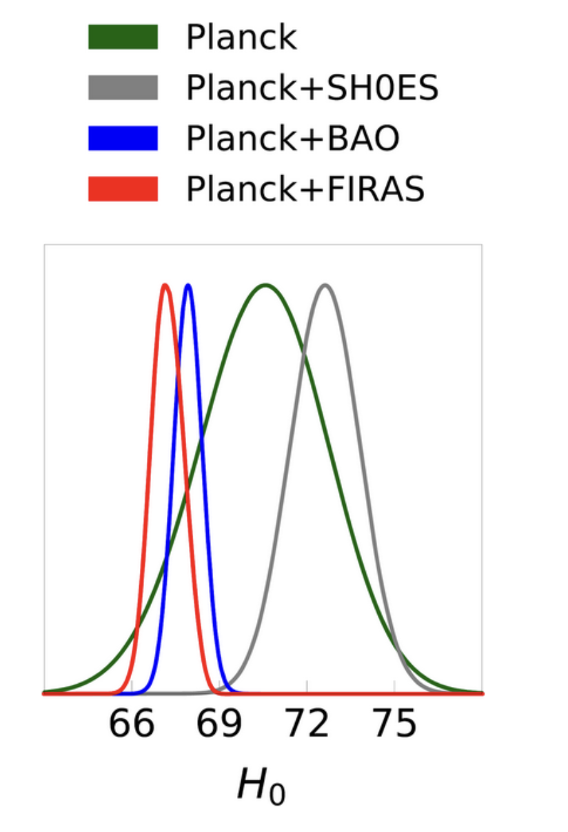
reading about H0, from early time cosmology and late time cosmology
Is the Hubble Tension actually a Temperature Tension? | astrobites
From CMB: T0 + anisotropical fluctuations = H0, T0 is a prior measured by other probes
Tension may come from different prior assumptions of T0.
Using BAO as an independent referee for T0:
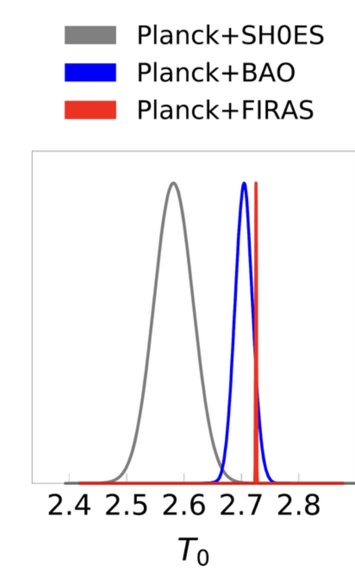
Using Planck only to find T0, then H0:
12-16
scarlet
My code actually did not take into the "turn-on" point for SN
After fixing it, it looks better, but still bright. Dan suggests do this for a star like object.
12-13
scarlet:
Working on multiple images:
#question
- Does the order of input images matter?
- I don't know how they deal with image that only has the galaxy
- Does pointing mean mjd?
from the group meeting:
- Maybe it's due to not setting up correctly about the turn on (where SN turns on)
- From the group meeting: fit a star (constant source) to it
observations_sc2[0], [1], [2] :rendered model
parametrization:
Total length
Scarlet2
- Rebuild scarlet2 environment on dcc
- Find more Roman images:
|filter|pointing|sca|
|---|---|---|
|str4|int64|int64|
|---|---|---|
|Y106|50188|18|
|Y106|50573|18|
|Y106|52118|18|
|Y106|54827|18|
- scarlet1 needs to be installed by git-clone method from their documentation page, and needs a further installation of peigen, and pybind11
- sep cannot work with numpy 2.xx, downgraded to 1.26
Current working scarlet2 environment and python version:
python: Python 3.10.15
# packages in environment at /opt/homebrew/anaconda3/envs/scarlet2:
#
# Name Version Build Channel
absl-py 2.1.0 pypi_0 pypi
anyio 3.7.1 pyhd8ed1ab_0 conda-forge
aom 3.9.1 h7bae524_0 conda-forge
appnope 0.1.4 pyhd8ed1ab_0 conda-forge
argon2-cffi 23.1.0 pyhd8ed1ab_0 conda-forge
argon2-cffi-bindings 21.2.0 py310h493c2e1_5 conda-forge
arviz 0.11.2 pyhd3eb1b0_0
asciitree 0.3.3 py_2 conda-forge
astropy 6.1.4 py310hae04be4_0 conda-forge
astropy-healpix 1.0.3 py310hae04be4_2 conda-forge
astropy-iers-data 0.2024.10.7.0.32.46 pyhd8ed1ab_0 conda-forge
asttokens 2.0.5 pyhd3eb1b0_0 anaconda
attrs 24.2.0 pyh71513ae_0 conda-forge
autograd 1.7.0 pypi_0 pypi
aws-c-auth 0.7.31 h14f56dd_2 conda-forge
aws-c-cal 0.7.4 hd45b2be_2 conda-forge
aws-c-common 0.9.29 h7ab814d_0 conda-forge
aws-c-compression 0.2.19 hd45b2be_2 conda-forge
aws-c-event-stream 0.4.3 hdf5079d_4 conda-forge
aws-c-http 0.8.10 h4588aaf_2 conda-forge
aws-c-io 0.14.19 h5ad5fc2_1 conda-forge
aws-c-mqtt 0.10.7 hbe077eb_2 conda-forge
aws-c-s3 0.6.7 h86d2b7d_0 conda-forge
aws-c-sdkutils 0.1.19 hd45b2be_4 conda-forge
aws-checksums 0.1.20 hd45b2be_1 conda-forge
aws-crt-cpp 0.28.3 h4f9f7e0_8 conda-forge
aws-sdk-cpp 1.11.407 h880863c_1 conda-forge
azure-core-cpp 1.13.0 hd01fc5c_0 conda-forge
azure-identity-cpp 1.8.0 h13ea094_2 conda-forge
azure-storage-blobs-cpp 12.12.0 hfde595f_0 conda-forge
azure-storage-common-cpp 12.7.0 hcf3b6fd_1 conda-forge
azure-storage-files-datalake-cpp 12.11.0 h082e32e_1 conda-forge
babel 2.14.0 pyhd8ed1ab_0 conda-forge
beautifulsoup4 4.12.3 pyha770c72_0 conda-forge
bleach 6.1.0 pyhd8ed1ab_0 conda-forge
blosc 1.21.6 h5499902_0 conda-forge
bokeh 3.6.0 pyhd8ed1ab_0 conda-forge
brotli 1.1.0 hd74edd7_2 conda-forge
brotli-bin 1.1.0 hd74edd7_2 conda-forge
brotli-python 1.1.0 py310hb4ad77e_2 conda-forge
brunsli 0.1 h9f76cd9_0 conda-forge
bzip2 1.0.8 h99b78c6_7 conda-forge
c-ares 1.34.3 h5505292_1 conda-forge
c-blosc2 2.14.3 ha57e6be_0 conda-forge
ca-certificates 2024.9.24 hca03da5_0 anaconda
certifi 2024.8.30 pyhd8ed1ab_0 conda-forge
cffi 1.17.1 py310h497396d_0 conda-forge
cftime 1.6.4 py310hae04be4_1 conda-forge
charls 2.4.2 h13dd4ca_0 conda-forge
charset-normalizer 3.4.0 pyhd8ed1ab_0 conda-forge
chex 0.1.87 pypi_0 pypi
click 8.1.7 unix_pyh707e725_0 conda-forge
cloudpickle 3.1.0 pyhd8ed1ab_1 conda-forge
cmasher 1.8.0 pypi_0 pypi
colorspacious 1.1.2 pypi_0 pypi
comm 0.2.2 pyhd8ed1ab_0 conda-forge
contourpy 1.3.0 py310h6000651_2 conda-forge
corner 2.2.2 pyhd8ed1ab_0 conda-forge
cycler 0.12.1 pyhd8ed1ab_0 conda-forge
cytoolz 1.0.0 py310h493c2e1_1 conda-forge
dask 2024.8.1 pyhd8ed1ab_0 conda-forge
dask-core 2024.8.1 pyhd8ed1ab_0 conda-forge
dask-expr 1.1.11 pyhd8ed1ab_0 conda-forge
dav1d 1.2.1 hb547adb_0 conda-forge
debugpy 1.8.7 py310hb4ad77e_0 conda-forge
decorator 5.1.1 pyhd3eb1b0_0 anaconda
defusedxml 0.7.1 pyhd8ed1ab_0 conda-forge
diffrax 0.6.0 pypi_0 pypi
distrax 0.1.5 pypi_0 pypi
distributed 2024.8.1 pyhd8ed1ab_0 conda-forge
dm-tree 0.1.8 pypi_0 pypi
einops 0.8.0 pypi_0 pypi
entrypoints 0.4 pyhd8ed1ab_0 conda-forge
equinox 0.11.8 pypi_0 pypi
etils 1.10.0 pypi_0 pypi
exceptiongroup 1.2.2 pyhd8ed1ab_0 conda-forge
executing 2.1.0 pypi_0 pypi
fasteners 0.17.3 pyhd8ed1ab_0 conda-forge
fonttools 4.54.1 py310h5799be4_1 conda-forge
freetype 2.12.1 hadb7bae_2 conda-forge
fsspec 2024.10.0 pyhff2d567_0 conda-forge
future 1.0.0 pypi_0 pypi
galaxygrad 0.1.8 pypi_0 pypi
galsim 2.6.1 pypi_0 pypi
gast 0.6.0 pypi_0 pypi
geos 3.13.0 hf9b8971_0 conda-forge
gflags 2.2.2 hf9b8971_1005 conda-forge
giflib 5.2.2 h93a5062_0 conda-forge
glog 0.7.1 heb240a5_0 conda-forge
h2 4.1.0 pyhd8ed1ab_0 conda-forge
hdf4 4.2.15 h2ee6834_7 conda-forge
hdf5 1.14.3 nompi_ha698983_108 conda-forge
hpack 4.0.0 pyh9f0ad1d_0 conda-forge
hyperframe 6.0.1 pyhd8ed1ab_0 conda-forge
icu 75.1 hfee45f7_0 conda-forge
idna 3.10 pyhd8ed1ab_0 conda-forge
imagecodecs 2024.1.1 py310hd5c6020_4 conda-forge
imageio 2.36.0 pyh12aca89_1 conda-forge
importlib-metadata 8.5.0 pyha770c72_0 conda-forge
importlib_metadata 8.5.0 hd8ed1ab_0 conda-forge
importlib_resources 6.4.5 pyhd8ed1ab_0 conda-forge
ipykernel 6.29.5 pyh57ce528_0 conda-forge
ipython 8.28.0 pyh707e725_0 conda-forge
ipython_genutils 0.2.0 pyhd8ed1ab_1 conda-forge
ipywidgets 8.1.5 pyhd8ed1ab_0 conda-forge
jax 0.4.28 pyhd8ed1ab_0 conda-forge
jaxlib 0.4.28 cpu_py310hc1dcdc7_0 conda-forge
jaxtyping 0.2.34 pypi_0 pypi
jedi 0.19.1 pyhd8ed1ab_0 conda-forge
jinja2 3.1.4 pyhd8ed1ab_0 conda-forge
json5 0.9.25 pyhd8ed1ab_0 conda-forge
jsonschema 4.23.0 pyhd8ed1ab_0 conda-forge
jsonschema-specifications 2024.10.1 pyhd8ed1ab_0 conda-forge
jupyter 1.1.1 pyhd8ed1ab_0 conda-forge
jupyter_client 7.1.2 pyhd3eb1b0_0 anaconda
jupyter_console 6.6.3 pyhd8ed1ab_0 conda-forge
jupyter_core 5.7.2 pyh31011fe_1 conda-forge
jupyter_server 1.24.0 pyhd8ed1ab_0 conda-forge
jupyterlab 3.5.3 pyhd8ed1ab_0 conda-forge
jupyterlab_pygments 0.3.0 pyhd8ed1ab_0 conda-forge
jupyterlab_server 2.27.3 pyhd8ed1ab_0 conda-forge
jupyterlab_widgets 3.0.13 pyhd8ed1ab_0 conda-forge
jxrlib 1.1 h93a5062_3 conda-forge
kiwisolver 1.4.7 py310h7306fd8_0 conda-forge
krb5 1.21.3 h237132a_0 conda-forge
lazy-loader 0.4 pyhd8ed1ab_1 conda-forge
lazy_loader 0.4 pyhd8ed1ab_1 conda-forge
lcms2 2.16 ha0e7c42_0 conda-forge
lerc 4.0.0 h9a09cb3_0 conda-forge
libabseil 20240116.2 cxx17_h00cdb27_1 conda-forge
libaec 1.1.3 hebf3989_0 conda-forge
libarrow 17.0.0 hc6a7651_16_cpu conda-forge
libarrow-acero 17.0.0 hf9b8971_16_cpu conda-forge
libarrow-dataset 17.0.0 hf9b8971_16_cpu conda-forge
libarrow-substrait 17.0.0 hbf8b706_16_cpu conda-forge
libavif16 1.1.1 ha4d98b1_1 conda-forge
libblas 3.9.0 24_osxarm64_openblas conda-forge
libbrotlicommon 1.1.0 hd74edd7_2 conda-forge
libbrotlidec 1.1.0 hd74edd7_2 conda-forge
libbrotlienc 1.1.0 hd74edd7_2 conda-forge
libcblas 3.9.0 24_osxarm64_openblas conda-forge
libcrc32c 1.1.2 hbdafb3b_0 conda-forge
libcurl 8.10.1 h13a7ad3_0 conda-forge
libcxx 19.1.1 ha82da77_0 conda-forge
libdeflate 1.20 h93a5062_0 conda-forge
libedit 3.1.20191231 hc8eb9b7_2 conda-forge
libev 4.33 h93a5062_2 conda-forge
libevent 2.1.12 h2757513_1 conda-forge
libexpat 2.6.3 hf9b8971_0 conda-forge
libffi 3.4.2 h3422bc3_5 conda-forge
libgfortran 5.0.0 13_2_0_hd922786_3 conda-forge
libgfortran5 13.2.0 hf226fd6_3 conda-forge
libgoogle-cloud 2.29.0 hfa33a2f_0 conda-forge
libgoogle-cloud-storage 2.29.0 h90fd6fa_0 conda-forge
libgrpc 1.62.2 h9c18a4f_0 conda-forge
libhwy 1.1.0 h2ffa867_0 conda-forge
libiconv 1.17 h0d3ecfb_2 conda-forge
libjpeg-turbo 3.0.0 hb547adb_1 conda-forge
libjxl 0.10.3 h44ef4fb_0 conda-forge
liblapack 3.9.0 24_osxarm64_openblas conda-forge
libmpdec 4.0.0 h99b78c6_0 conda-forge
libnetcdf 4.9.2 nompi_he469be0_114 conda-forge
libnghttp2 1.58.0 ha4dd798_1 conda-forge
libopenblas 0.3.27 openmp_h517c56d_1 conda-forge
libparquet 17.0.0 hf0ba9ef_16_cpu conda-forge
libpng 1.6.44 hc14010f_0 conda-forge
libprotobuf 4.25.3 hc39d83c_1 conda-forge
libre2-11 2023.09.01 h7b2c953_2 conda-forge
libsodium 1.0.20 h99b78c6_0 conda-forge
libsqlite 3.46.1 hc14010f_0 conda-forge
libssh2 1.11.0 h7a5bd25_0 conda-forge
libthrift 0.20.0 h64651cc_1 conda-forge
libtiff 4.6.0 h07db509_3 conda-forge
libutf8proc 2.8.0 h1a8c8d9_0 conda-forge
libwebp-base 1.4.0 h93a5062_0 conda-forge
libxcb 1.17.0 hdb1d25a_0 conda-forge
libxml2 2.12.7 h01dff8b_4 conda-forge
libzip 1.11.1 hfc4440f_0 conda-forge
libzlib 1.3.1 h8359307_2 conda-forge
libzopfli 1.0.3 h9f76cd9_0 conda-forge
lineax 0.0.7 pypi_0 pypi
llvm-openmp 19.1.1 h6cdba0f_0 conda-forge
locket 1.0.0 pyhd8ed1ab_0 conda-forge
lsstdesc-coord 1.3.0 pypi_0 pypi
lz4 4.3.3 py310hc798581_1 conda-forge
lz4-c 1.9.4 hb7217d7_0 conda-forge
markupsafe 3.0.2 py310h5799be4_0 conda-forge
matplotlib-base 3.9.2 py310h2a20ac7_1 conda-forge
matplotlib-inline 0.1.2 pyhd3eb1b0_2 anaconda
mistune 3.0.2 pyhd8ed1ab_0 conda-forge
ml_dtypes 0.5.0 py310hfd37619_0 conda-forge
msgpack-python 1.1.0 py310h7306fd8_0 conda-forge
multipledispatch 1.0.0 pypi_0 pypi
munkres 1.1.4 pyh9f0ad1d_0 conda-forge
nbclassic 1.1.0 pyhd8ed1ab_0 conda-forge
nbclient 0.10.0 pyhd8ed1ab_0 conda-forge
nbconvert-core 7.16.4 pyhd8ed1ab_1 conda-forge
nbformat 5.10.4 pyhd8ed1ab_0 conda-forge
ncurses 6.5 h7bae524_1 conda-forge
nest-asyncio 1.5.1 pyhd3eb1b0_0 anaconda
netcdf4 1.7.2 nompi_py310h150c015_101 conda-forge
networkx 3.4.2 pyhd8ed1ab_0 conda-forge
notebook 6.5.7 pyha770c72_0 conda-forge
notebook-shim 0.2.4 pyhd8ed1ab_0 conda-forge
numcodecs 0.13.1 py310h3420790_0 conda-forge
numpy 1.26.4 py310hd45542a_0 conda-forge
numpyro 0.15.3 pypi_0 pypi
openjpeg 2.5.2 h9f1df11_0 conda-forge
openssl 3.4.0 h39f12f2_0 conda-forge
opt-einsum 3.4.0 hd8ed1ab_0 conda-forge
opt_einsum 3.4.0 pyhd8ed1ab_0 conda-forge
optax 0.2.3 pypi_0 pypi
optimistix 0.0.9 pypi_0 pypi
orc 2.0.2 h75dedd0_0 conda-forge
packaging 24.1 pyhd8ed1ab_0 conda-forge
pandas 2.2.3 py310hfd37619_1 conda-forge
pandocfilters 1.5.0 pyhd8ed1ab_0 conda-forge
parso 0.8.3 pyhd3eb1b0_0 anaconda
partd 1.4.2 pyhd8ed1ab_0 conda-forge
peigen 0.0.9 pypi_0 pypi
pexpect 4.8.0 pyhd3eb1b0_3 anaconda
photutils 2.0.2 pypi_0 pypi
pickleshare 0.7.5 pyhd3eb1b0_1003 anaconda
pillow 10.4.0 py310h383043f_1 conda-forge
pip 24.2 pyh8b19718_1 conda-forge
pkgutil-resolve-name 1.3.10 pyhd8ed1ab_1 conda-forge
platformdirs 4.3.6 pyhd8ed1ab_0 conda-forge
prometheus_client 0.21.0 pyhd8ed1ab_0 conda-forge
prompt-toolkit 3.0.48 pyha770c72_0 conda-forge
prompt_toolkit 3.0.48 hd8ed1ab_0 conda-forge
proxmin 0.6.12 pypi_0 pypi
psutil 6.1.0 py310hf9df320_0 conda-forge
pthread-stubs 0.4 hd74edd7_1002 conda-forge
ptyprocess 0.7.0 pyhd3eb1b0_2 anaconda
pure_eval 0.2.2 pyhd3eb1b0_0 anaconda
pyarrow 17.0.0 py310h24597f5_2 conda-forge
pyarrow-core 17.0.0 py310hc17921c_2_cpu conda-forge
pyarrow-hotfix 0.6 pyhd8ed1ab_0 conda-forge
pybind11 2.13.6 pyh085cc03_1 conda-forge
pybind11-global 2.13.6 pyh085cc03_1 conda-forge
pycparser 2.22 pyhd8ed1ab_0 conda-forge
pyerfa 2.0.1.4 py310hae04be4_2 conda-forge
pygments 2.11.2 pyhd3eb1b0_0 anaconda
pyobjc-core 10.3.1 py310hb3dec1a_1 conda-forge
pyobjc-framework-cocoa 10.3.1 py310hb3dec1a_1 conda-forge
pyparsing 3.1.4 pyhd8ed1ab_0 conda-forge
pysocks 1.7.1 pyha2e5f31_6 conda-forge
python 3.10.15 hdce6c4c_2_cpython conda-forge
python-dateutil 2.9.0 pyhd8ed1ab_0 conda-forge
python-fastjsonschema 2.20.0 pyhd8ed1ab_0 conda-forge
python-tzdata 2024.2 pyhd8ed1ab_0 conda-forge
python_abi 3.10 5_cp310 conda-forge
pytz 2024.1 pyhd8ed1ab_0 conda-forge
pywavelets 1.7.0 py310h003b70b_2 conda-forge
pyyaml 6.0.2 py310h493c2e1_1 conda-forge
pyzmq 26.2.0 py310h82ef58e_3 conda-forge
qhull 2020.2 h420ef59_5 conda-forge
rav1e 0.6.6 h69fbcac_2 conda-forge
re2 2023.09.01 h4cba328_2 conda-forge
readline 8.2 h92ec313_1 conda-forge
referencing 0.35.1 pyhd8ed1ab_0 conda-forge
reproject 0.14.0 py310hb3e58dc_0 conda-forge
requests 2.32.3 pyhd8ed1ab_0 conda-forge
rpds-py 0.20.0 py310h7a930dc_1 conda-forge
scarlet 1.0.1+g3ce064d pypi_0 pypi
scarlet2 0.2.0 pypi_0 pypi
scikit-image 0.24.0 py310h3420790_3 conda-forge
scipy 1.14.1 py310hc05a576_1 conda-forge
send2trash 1.8.3 pyh31c8845_0 conda-forge
sep 1.2.1 py310h280b8fa_2 conda-forge
setuptools 71.1.0 pypi_0 pypi
shapely 2.0.6 py310h6b3522b_2 conda-forge
six 1.16.0 pyh6c4a22f_0 conda-forge
snappy 1.2.1 h98b9ce2_1 conda-forge
sniffio 1.3.1 pyhd8ed1ab_0 conda-forge
sortedcontainers 2.4.0 pyhd8ed1ab_0 conda-forge
soupsieve 2.5 pyhd8ed1ab_1 conda-forge
stack_data 0.2.0 pyhd3eb1b0_0 anaconda
svt-av1 2.2.1 ha39b806_0 conda-forge
tblib 3.0.0 pyhd8ed1ab_0 conda-forge
tensorflow-probability 0.24.0 pypi_0 pypi
terminado 0.18.1 pyh31c8845_0 conda-forge
tifffile 2024.9.20 pyhd8ed1ab_0 conda-forge
tinycss2 1.3.0 pyhd8ed1ab_0 conda-forge
tk 8.6.13 h5083fa2_1 conda-forge
tomli 2.0.2 pyhd8ed1ab_0 conda-forge
toolz 1.0.0 pyhd8ed1ab_0 conda-forge
tornado 6.4.1 py310h493c2e1_1 conda-forge
tqdm 4.66.5 pypi_0 pypi
traitlets 5.14.3 pyhd8ed1ab_0 conda-forge
typeguard 2.13.3 pypi_0 pypi
typing-extensions 4.12.2 hd8ed1ab_0 conda-forge
typing_extensions 4.12.2 pyha770c72_0 conda-forge
tzdata 2024b hc8b5060_0 conda-forge
unicodedata2 15.1.0 py310hf9df320_1 conda-forge
urllib3 2.2.3 pyhd8ed1ab_0 conda-forge
varname 0.13.5 pypi_0 pypi
wcwidth 0.2.5 pyhd3eb1b0_0 anaconda
webencodings 0.5.1 pyhd8ed1ab_2 conda-forge
websocket-client 1.8.0 pyhd8ed1ab_0 conda-forge
wheel 0.44.0 pyhd8ed1ab_0 conda-forge
widgetsnbextension 4.0.13 pyhd8ed1ab_0 conda-forge
xarray 2024.9.0 pyhd8ed1ab_1 conda-forge
xorg-libxau 1.0.11 hd74edd7_1 conda-forge
xorg-libxdmcp 1.1.5 hd74edd7_0 conda-forge
xyzservices 2024.9.0 pyhd8ed1ab_0 conda-forge
xz 5.2.6 h57fd34a_0 conda-forge
yaml 0.2.5 h3422bc3_2 conda-forge
zarr 2.18.3 pyhd8ed1ab_0 conda-forge
zeromq 4.3.5 h9f5b81c_6 conda-forge
zfp 1.0.1 h1c5d8ea_2 conda-forge
zict 3.0.0 pyhd8ed1ab_0 conda-forge
zipp 3.20.2 pyhd8ed1ab_0 conda-forge
zlib 1.3.1 h8359307_2 conda-forge
zlib-ng 2.0.7 h1a8c8d9_0 conda-forge
zstandard 0.23.0 py310h2665a74_1 conda-forge
zstd 1.5.6 hb46c0d2_0 conda-forge
12-12
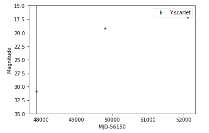
Progress!! First light curve
It looks too bright. But I will try with multiple images.
[Fixed] scene.morphology has no attribute center:
change from
p = scene_.sources[indtransient].morphology.center
to
p = scene_.sources[indtransient].center
[Fixed] Jax issue:
ValueError: Expected None, got Array([ 5., 34.], dtype=float32).

In previous releases of JAX, flatten-up-to used to consider None to be a tree-prefix of non-None values. To obtain the previous behavior, you can usually write:
  jax.tree.map(lambda x, y: None if x is None else f(x, y), a, b, is_leaf=lambda x: x is None)
test_quickstart.py · Issue #87 · pmelchior/scarlet2 · GitHub
Forcing jax and jaxlib to version 0.4.28 resolves the issue and allows test_quickstart.py to run successfully.
Model after fitting:
12-11
Meeting with Ben
#Parametrization:
Fixed parameters: welded length (d_wel)
Measure from the other side of the tube to the end of the flange (d1)
Dimension of the Flange (d2)
Tube length is derived from d1- d2 + de_wel
Work on these two side, (with the welded part), and then work on the total length
My updates:
Found a better way to type things in
Only trouble is to figure out which dimension is which (the dimension may be drawn on a different plane)
You can't change section view when editing equations
Some tricks to make it easier: click parameter from the annotation tree, from "top plane" or other plane sub tree.
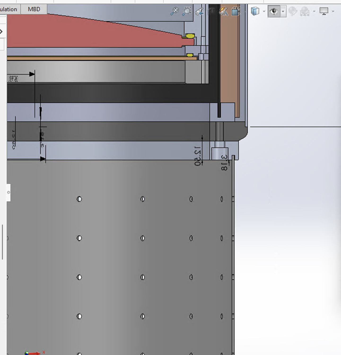
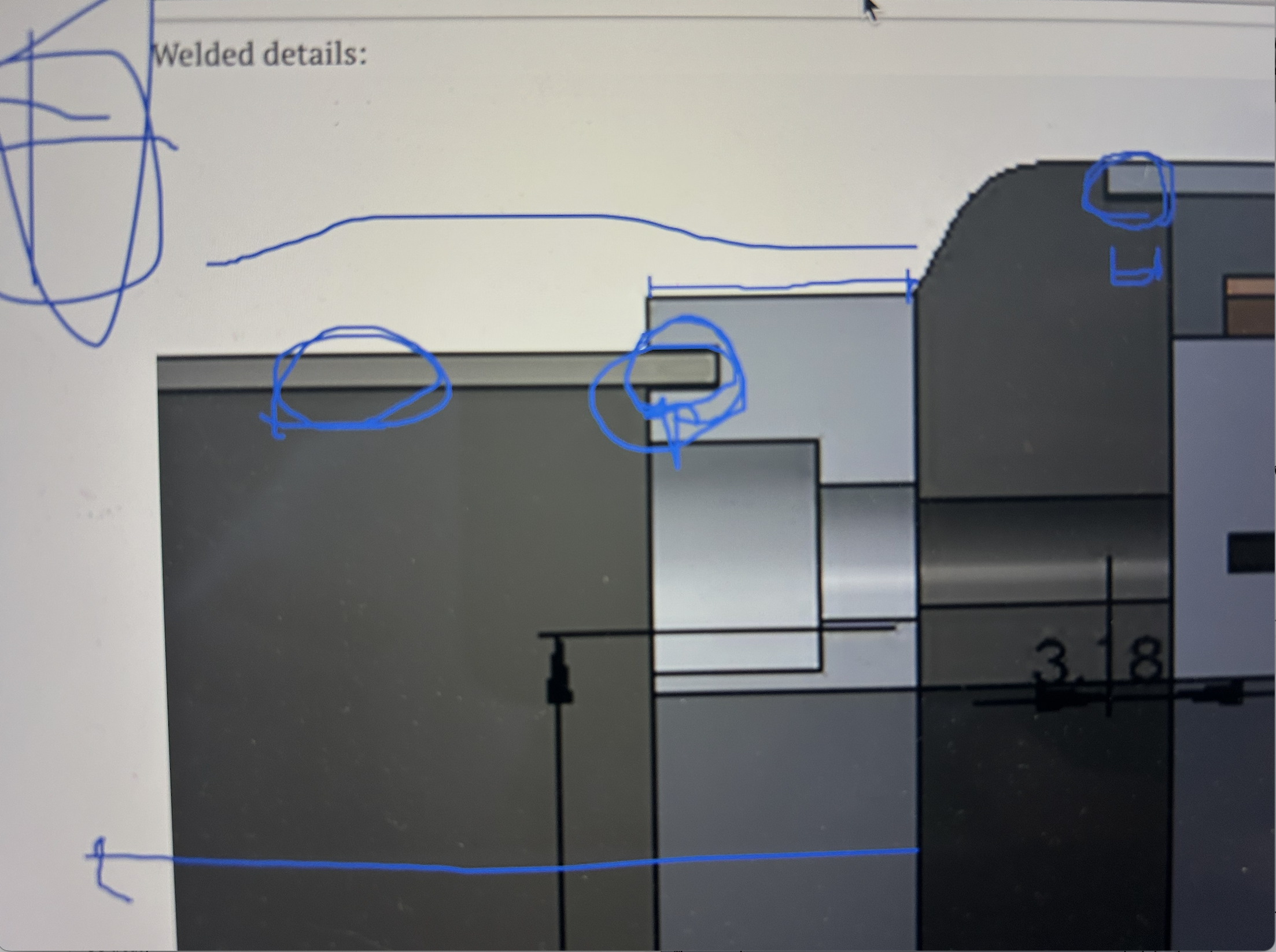
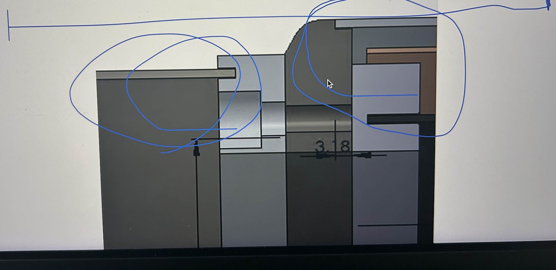
Welded details:
12-10
Continue with Scarlet 2 on Roman images. Going through the code carefully.
Progress: Can extract sources now.
To do: need the last fitting process. It'll stuck...
#question
- Why mjd_on (where transient is turned on) is set to be 56160
if mjd>56160:
            channels_on.append(channel_sc2)
- Is knowing start_mjd important in doing the model?
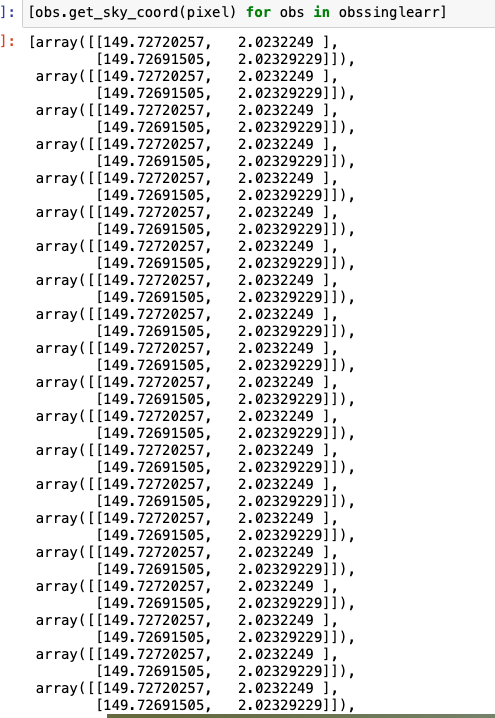
- What if different image detected different number of sources? Now it only uses the first image for retrieving the sources' ra_dec
ra_dec = [obs.get_sky_coord(pixel) for obs in obssinglearr][0]
- Why flux is 1.2 times, why 1.2?
flux = 1.2*np.copy(np.asarray(initialization.pixel_spectrum(observations_sc2, centerpix).data))
- PSF used so far is not from Roman, but just a fake one
- Priors are pretrained, on ZTF
- Imports:
HSC_ScoreNet32andZTF_ScoreNet32: Pretrained ScoreNet models for prior regularization.nn.ScorePrior: Defines a prior to encourage physically realistic source models.
- Prior:
ZTF_ScoreNet32is used as a prior to regularize source morphologies based on data-driven knowledge (e.g., galaxy shapes).
makeCatalog function
- Imports:
The makeCatalog function is designed to generate a catalog of sources, estimate background flux and noise levels, and create a detection image for subsequent analysis.
- If only once source is detected, duplicate the ra_dec. Abandoned... no need
- The error: Pixel value out of bound:
Solution: centerpix mixed with center.15 centerpix = jnp.asarray([pospix[1],pospix[0]]) 17 if i==indtransient: ---> 18 flux = np.asarray(initialization.pixel_spectrum(observations_sc2, center))[:,0] ValueError: Pixel coordinate expected, got [149 2]
Also need to change to the line offlux = 1.2*np.copy(np.asarray(initialization.pixel_spectrum(observations_sc2, centerpix).data)) - Changed Channel name to "Y" instead of "Y106"
wavelet-based detection?
Wavelet-based detection refers to using wavelet transforms to identify and enhance structures in an image at specific spatial scales. This technique is commonly applied in astrophysical image analysis because it allows the separation of sources (e.g., stars, galaxies) from noise or background fluctuations by isolating features of interest based on their size and intensity.
It won't be ale to deblend two sources if they're close by
issue: only extract the first letter for the band pass (It's Y106)
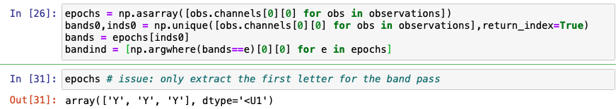
Example:
epochs = ['g', 'g', 'r', 'r', 'i', 'i']bands = ['g', 'r', 'i']bandind = [0, 0, 1, 1, 2, 2].
12-09
Working on Scarlet2 impletation on Roman images. Reading carefully about the paper, and want to know why mine only detect one source
Epoch?
channel and channle_sc2?

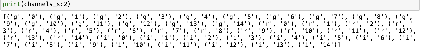
The numbers appended to the band names (e.g., g0, g1, r2, i14) typically represent the epoch or time index for observations within that band. Here's a detailed explanation:
Interpretation of the Channel Labels:
-
Band Letter (
g,r,i):- Represents the photometric filter used for the observation.
- Commonly, these correspond to the standard LSST or similar photometric bands:
g: Green (~475 nm)r: Red (~622 nm)i: Infrared (~754 nm)
-
Number (
0,1,2, ...):- Indicates the time sequence or epoch of the observation within that band.
- For example:
g0: The first observation in thegband.g1: The second observation in thegband.r3: The fourth observation in therband.i14: The 15th observation in theiband.
Purpose of Numbering:
- The numbering ensures that every image has a unique identifier even if multiple images exist for the same band.
- It is particularly useful for time-domain analyses, where observations from multiple epochs must be distinguished for creating light curves.
How the Code Assigns These Labels:
The numbers are appended using the ind variable, which is derived from the enumerate() function when looping over image files for each band:
for ind, (img, psf) in enumerate(zip(imageout, psfs)):
    channel = [band+str(ind)]  # Appends the band name with the index
    channels.append(band+str(ind))
Here:
bandis the photometric filter (e.g.,g,r,i).indis the index of the file in the list of images for the current band, starting from 0.
Application in Modeling:
These labels are used:
- To Track Observations: The unique channel identifiers allow the code to associate data, PSF, and metadata for each observation.
- For Multi-Epoch Analysis: By combining data across channels, the transient's variability can be modeled, and light curves can be extracted.
12-03
Measuring Density Parameters
Accurate determination of density parameters relies on multiple observational techniques:
1. Cosmic Microwave Background (CMB)
- Role: Provides a snapshot of the early Universe, allowing precise measurements of Ω_total, Ωₘ, Ω_Λ, and Ωᵣ through temperature anisotropies and polarization patterns.
2. Type Ia Supernovae
- Role: Serve as "standard candles" to measure cosmic distances and expansion rates, crucial for determining Ω_Λ.
3. Baryon Acoustic Oscillations (BAO)
- Role: Act as a "standard ruler" to measure the scale of large-scale structures, informing Ωₘ and Ω_Λ.
4. Galaxy Clustering and Weak Gravitational Lensing
- Role: Probe the distribution of matter (both visible and dark) to constrain Ωₘ.
5. Big Bang Nucleosynthesis (BBN)
- Role: Predicts the abundances of light elements, constraining Ωᵦ.
EoS parameters and different probes
Constraining the equation of state (EoS) parameters for various components of the Universe—such as dark energy, dark matter, and radiation—is essential for understanding cosmic evolution and the ultimate fate of the cosmos. Observational probes are the primary tools through which cosmologists gather data to place these constraints. Below, we delve into five key observational probes and explore in detail how each contributes to constraining the EoS parameters of different cosmological components.
1. Type Ia Supernovae (SNe Ia)
Overview
Type Ia Supernovae are stellar explosions that occur in binary systems where a white dwarf accretes matter from a companion star until it reaches a critical mass, leading to a thermonuclear explosion. Due to their consistent peak luminosity, SNe Ia serve as "standard candles" for measuring cosmic distances.
How SNe Ia Constrain EoS Parameters
a. Measuring Cosmic Expansion History
-
Distance Modulus and Redshift:
- By measuring the apparent brightness (flux) of SNe Ia and knowing their intrinsic brightness (absolute magnitude), cosmologists calculate the distance modulus, which relates to the luminosity distance.
- Plotting distance modulus against redshift (( z )) provides insights into the expansion rate of the Universe over time.
-
Luminosity Distance Relation:
- The relationship between luminosity distance (( d_L )) and redshift is sensitive to the Hubble parameter (( H(z) )), which in turn depends on the EoS parameters of various components.
- The EoS of dark energy (( w )) affects how ( H(z) ) evolves, thereby influencing the observed brightness of SNe Ia at different redshifts.
b. Detecting Accelerated Expansion
- Discovery of Dark Energy:
- Observations of distant SNe Ia revealed that the Universe's expansion is accelerating, a phenomenon attributed to dark energy with ( w \approx -1 ).
- Precise measurements of SNe Ia distances across a range of redshifts help refine the value of ( w ) and assess its consistency with the cosmological constant (( w = -1 )).
c. Parameter Fitting and Constraints
- Statistical Analysis:
- By fitting the observed distance-redshift data to cosmological models, SNe Ia constrain combinations of EoS parameters, particularly for dark energy (( w )) and the matter density (( \Omega_m )).
- Confidence Intervals: Bayesian and frequentist statistical methods are used to derive confidence intervals for ( w ), often resulting in constraints like ( w = -1 \pm 0.1 ).
Limitations and Systematics
-
Calibration Uncertainties:
- Accurate calibration of SNe Ia luminosities is crucial. Systematic errors in calibration can bias EoS constraints.
-
Evolution Effects:
- Potential evolution in SNe Ia properties over cosmic time could affect distance measurements, impacting ( w ) estimates.
Impact on EoS Parameters
-
Primary Constraint on Dark Energy (( w )):
- SNe Ia are most sensitive to the EoS parameter of dark energy (( w )), providing one of the strongest direct constraints on its value.
-
Degeneracies:
- While SNe Ia effectively constrain ( w ), they often need to be combined with other probes to break parameter degeneracies, such as those between ( w ) and ( \Omega_m ).
2. Cosmic Microwave Background (CMB) Radiation
Overview
The Cosmic Microwave Background is the afterglow radiation from the Big Bang, providing a snapshot of the Universe when it was approximately 380,000 years old. The CMB contains minute temperature and polarization anisotropies that encode rich information about the early Universe's conditions.
How CMB Constrains EoS Parameters
a. Geometrical Constraints
- Angular Scale of Acoustic Peaks:
- The position of the first acoustic peak in the CMB power spectrum is sensitive to the geometry of the Universe, which depends on the total density parameter (( \Omega_{\text{total}} )).
- A flat Universe (( \Omega_{\text{total}} = 1 )) aligns the observed peak positions with theoretical predictions, indirectly constraining ( w ) by fixing the spatial curvature.
b. Integrated Sachs-Wolfe (ISW) Effect
- Late-Time ISW Effect:
- Occurs when CMB photons traverse evolving gravitational potentials due to dark energy's influence on cosmic expansion.
- Enhances large-scale temperature anisotropies, providing constraints on ( w ) by measuring the rate of Universe's acceleration.
c. Damping Tail and Reionization
-
Silk Damping:
- The damping of small-scale anisotropies due to photon diffusion affects constraints on the radiation density (( \Omega_r )) and indirectly on dark energy through the overall energy budget.
-
Optical Depth (( \tau )):
- The degree of reionization affects polarization measurements, influencing constraints on dark energy's EoS through its impact on the growth of structures.
d. Parameter Degeneracies and Complementarity
- Breaking Degeneracies:
- CMB data alone may exhibit degeneracies between ( w ) and other parameters (e.g., ( H_0 ), ( \Omega_m )). However, when combined with other probes like SNe Ia and BAO, these degeneracies can be broken, leading to tighter constraints on ( w ).
e. Acoustic Oscillations and Early Universe Physics
- Sound Horizon:
- Precise measurements of the sound horizon scale from the CMB provide a "standard ruler" that complements BAO measurements, enhancing constraints on ( w ).
Impact on EoS Parameters
-
Indirect Constraints on Dark Energy (( w )):
- While the CMB is primarily sensitive to early Universe parameters, its influence on the integrated expansion history allows it to place indirect constraints on dark energy's EoS.
-
Combined Constraints:
- CMB data significantly improves the precision of ( w ) when combined with low-redshift probes, making it a cornerstone for modern cosmological parameter estimation.
3. Baryon Acoustic Oscillations (BAO)
Overview
Baryon Acoustic Oscillations are periodic fluctuations in the density of the visible baryonic matter of the Universe caused by acoustic waves in the early plasma. These oscillations leave an imprint on the large-scale structure of the Universe, acting as a "standard ruler" for cosmological distance measurements.
How BAO Constrains EoS Parameters
a. Standard Ruler for Distance Measurements
- Scale of BAO:
- The characteristic scale of BAO (~150 Mpc) is imprinted in the distribution of galaxies and can be measured in both the radial and transverse directions.
- Comparing the observed BAO scale with the predicted physical scale from the CMB allows for precise measurements of the angular diameter distance (( D_A(z) )) and the Hubble parameter (( H(z) )) at different redshifts.
b. Angular and Radial BAO Measurements
-
Transverse BAO:
- Measures the angular size of the BAO feature, constraining ( D_A(z) ).
-
Radial BAO:
- Measures the line-of-sight scale, constraining ( H(z) ).
c. Sensitivity to Dark Energy EoS (( w ))
- Expansion History:
- The relationship between ( D_A(z) ), ( H(z) ), and redshift ( z ) is sensitive to the dark energy EoS parameter (( w )).
- By precisely measuring ( D_A(z) ) and ( H(z) ), BAO provides constraints on how ( w ) affects the expansion rate over cosmic time.
d. Redshift Dependence
- Multiple Redshift Surveys:
- Conducting BAO measurements at various redshifts enhances the ability to track the evolution of ( w ) and detect any possible variation over time.
e. Complementarity with Other Probes
- Combined Constraints:
- BAO data complements SNe Ia and CMB observations by providing independent distance measurements, thereby strengthening overall constraints on ( w ).
Impact on EoS Parameters
-
Precise Measurement of Dark Energy (( w )):
- BAO offers one of the most robust methods for constraining ( w ), especially when combined with CMB and SNe Ia data.
-
Enhanced Precision:
- The ability to measure ( D_A(z) ) and ( H(z) ) with high precision leads to tighter bounds on ( w ), often reducing uncertainties to a few percent.
-
Constraining ( w ) Evolution:
- By analyzing BAO at different redshifts, cosmologists can investigate whether ( w ) remains constant or evolves, providing insights into the nature of dark energy.
4. Weak Gravitational Lensing
Overview
Weak gravitational lensing refers to the subtle distortion of the images of distant galaxies due to the bending of light by intervening mass distributions (both visible and dark matter). By statistically analyzing these distortions, cosmologists can map the matter distribution in the Universe.
How Weak Lensing Constrains EoS Parameters
a. Mapping Dark Matter Distribution
-
Mass Distribution:
- Weak lensing provides detailed maps of the total matter distribution, including dark matter, by measuring the shear (distortion) and convergence (magnification) of background galaxy images.
-
Growth of Structures:
- The rate at which structures (e.g., galaxy clusters) grow over time is influenced by the presence of dark energy, making weak lensing sensitive to ( w ).
b. Sensitivity to Dark Energy and Modified Gravity
-
Impact on Growth Rate:
- Dark energy affects the rate of cosmic expansion, which in turn influences the growth rate of cosmic structures. Weak lensing measurements of structure growth can thus constrain ( w ).
-
Distinguishing Dark Energy from Modified Gravity:
- By comparing the lensing-derived matter distribution with other probes (e.g., galaxy clustering), weak lensing can help distinguish between dark energy and modifications to General Relativity as explanations for cosmic acceleration.
c. Tomographic Weak Lensing
- Redshift Binning:
- Dividing source galaxies into redshift bins (tomography) allows for three-dimensional mapping of the matter distribution, enhancing sensitivity to the time evolution of ( w ).
d. Statistical Analysis
- Shear Correlation Functions:
- Analyzing the statistical properties of shear measurements (e.g., two-point correlation functions) provides constraints on the amplitude and growth rate of matter fluctuations, linked to ( w ).
e. Synergy with Other Probes
- Cross-Correlation:
- Combining weak lensing with other probes like BAO and CMB improves constraints on ( w ) by leveraging different sensitivities and breaking parameter degeneracies.
Impact on EoS Parameters
-
Constraining Dark Energy (( w )):
- Weak lensing is particularly effective at constraining the growth index, which is sensitive to ( w ), thereby providing indirect constraints on its value.
-
Enhanced Sensitivity to ( w ) Evolution:
- Tomographic analyses allow for the exploration of potential time variations in ( w ), offering insights into dynamic dark energy models.
-
Robustness Against Systematics:
- While weak lensing measurements are powerful, they require careful control of systematic uncertainties (e.g., intrinsic alignments, measurement biases) to ensure accurate ( w ) constraints.
5. Large-Scale Structure (LSS) Surveys
Overview
Large-Scale Structure refers to the distribution of matter on scales of millions of light-years, encompassing galaxies, galaxy clusters, filaments, and voids. LSS surveys map these structures, providing vital information about the Universe's composition and evolution.
How LSS Constrains EoS Parameters
a. Galaxy Clustering and Power Spectrum
-
Clustering Statistics:
- Analyzing the two-point correlation function or the power spectrum of galaxy distributions reveals information about the underlying matter density and its fluctuations, both of which are influenced by ( w ).
-
Shape of the Power Spectrum:
- The shape and amplitude of the power spectrum are sensitive to the matter density (( \Omega_m )) and the dark energy EoS parameter (( w )) through their effects on growth rates and the expansion history.
b. Redshift-Space Distortions (RSD)
- Measuring Growth Rate:
- RSD arise from the peculiar velocities of galaxies and provide direct measurements of the growth rate of cosmic structures.
- The growth rate is sensitive to both ( \Omega_m ) and ( w ), allowing LSS surveys to constrain ( w ) by measuring how structures grow over time.
c. Halo Occupation Distribution (HOD) Models
- Linking Galaxies to Dark Matter Halos:
- HOD models describe how galaxies populate dark matter halos. By understanding this relationship, LSS surveys can better interpret clustering data, refining constraints on ( w ).
d. Alcock-Paczynski (AP) Test
- Geometric Test:
- The AP test compares the observed shapes of structures (e.g., galaxy clusters) in redshift and angular dimensions to their expected shapes based on cosmological models.
- Deviations from expected shapes can constrain ( w ) by assessing the underlying cosmology's impact on observed geometries.
e. Cross-Correlation with Other Probes
- Multi-Probe Analyses:
- Combining LSS data with other probes like BAO, weak lensing, and CMB enhances the precision of ( w ) constraints by leveraging complementary information.
Impact on EoS Parameters
-
Direct Constraints on Dark Energy (( w )):
- By measuring the growth rate and clustering of galaxies, LSS surveys provide direct constraints on how dark energy influences structure formation, thereby constraining ( w ).
-
Breaking Parameter Degeneracies:
- LSS data help disentangle the effects of ( \Omega_m ) and ( w ), especially when combined with other probes like CMB and BAO.
-
Exploring ( w ) Evolution:
- High-redshift LSS surveys allow for the investigation of ( w )'s potential time evolution, offering insights into dynamic dark energy models.
Integrating Multiple Probes for Robust Constraints
While each observational probe offers unique strengths in constraining EoS parameters, their true power emerges when combined. Integrating data from Type Ia Supernovae, CMB, BAO, Weak Gravitational Lensing, and Large-Scale Structure Surveys allows cosmologists to:
-
Break Parameter Degeneracies:
- Different probes are sensitive to different combinations of parameters. Combining them helps isolate individual EoS parameters like ( w ).
-
Cross-Validate Results:
- Independent verification from multiple probes enhances the reliability of constraints and reduces systematic uncertainties.
-
Enhance Precision:
- Joint analyses significantly tighten confidence intervals, leading to more precise determinations of ( w ).
-
Probe Different Epochs:
- Probes like CMB inform about the early Universe, while SNe Ia and LSS surveys provide insights into the late-time Universe, offering a comprehensive view of ( w )'s impact across cosmic history.
Conclusion
Constraining the equation of state parameters for various cosmological components is a multifaceted endeavor that relies on diverse observational probes. Each probe—Type Ia Supernovae, Cosmic Microwave Background, Baryon Acoustic Oscillations, Weak Gravitational Lensing, and Large-Scale Structure Surveys—offers unique insights into different aspects of the Universe's composition and evolution. By leveraging the strengths of each and integrating their data, cosmologists can robustly constrain the EoS parameters, enhancing our understanding of dark energy, dark matter, and the overall dynamics of the cosmos. Ongoing and future surveys, with their increased precision and scope, promise to further refine these constraints, potentially unveiling new physics beyond the current ΛCDM paradigm.
11-30
LSST DESC white paper:
arxiv.org/pdf/1211.0310
Cosmology note book/lecture notes:
damtp.cam.ac.uk/user/tong/cosmo/cosmo.pdf
Index of /~pettini/Intro Cosmology
11-22
Issue:
Converted pixel coordinates: [2499.57313667 2878.4494142 ] Bounding box: Box(shape=(80, 80), origin=(0, 0))
SN pixel range outside bound:
Used original image wcs, but need the cutout wcs to put into Scarlet 2 frame
11-14
#toRead
aidantr.github.io/files/AI_innovation.pdf
Some decisions:
Simplified version of makeCatalog function: directly adding images, since we projected images before hand, and they are the same resolution
Debugging worked:
def align_dimension(data):
if data.ndim == 2:
data = np.expand_dims(data, axis=0)
return data
data_pre_peak_bkg_sub = align_dimension(data_pre_peak_bkg_sub)
data_peak_aligned = align_dimension(data_peak_aligned)
mask_pre_peak = align_dimension(mask_pre_peak)
mask_peak_aligned = align_dimension(mask_peak_aligned)
Before np.expand_dims is not in a function and the cell has been run for multiple times, making the dimension of data higher dimensional.
Progress: Able to construct observation object, and source detection
Next: Plot the detected sources, and
- reprojection issue (nan value encountered)
#scarlet
Issue with scarlet: current resolution: comment out that line
#toExplore
Use command in obsidian to automatically collect questions.
manage tags on obsidian
#question
Structure of enviroment , like bin folder, etc..
#shortcut #notes
To open the current Finder window in Terminal on a Mac, you can use the following shortcut:
- Press
Command (⌘) + Shift + .to show any hidden files if needed. - Then right-click in the Finder window (or on the folder icon in Finder), hold down the
Optionkey, and select Copy "Folder Name" as Pathname. - Open Terminal and type
cd, pressCommand (⌘) + Vto paste the path, and pressEnterto navigate to that folder.
Unable to compress files in window view
➡ shell command: zip -r compressed_folder.zip folder_name
11-11
With Bruno:
Step 1
Check the similaritiees between data set , DES and ZTF, and Elassticc
- check distribution of fluxes for each band, for both DES and Elasticc (frequency histogram)
- plot all light curves, stack with their peak time, normalize the flux, for
They should look the same
If they does not look the same: may explain the very bad behavior of transfer learning
If they looks the same, something goes wrong with the applying algorithm part, either it's normalization, or preporcessing, nan value has accidentally passed.... You need to massage your data.
Step 2
PariSNIP
Auto Encoder
Finding the clumps:
Clustering
t-SNe
UMAP
11-09
[To do]
[Note]
Summary of Questions
Python Basics and Class Structure
-
super().__init__in Subclassing:- Calls the initializer of the superclass to set up inherited attributes in a subclass, enabling reuse of initialization logic.
-
Purpose of
@abstractmethod:- Declares a method as abstract, requiring subclasses to implement it, defining a consistent interface across subclasses.
-
Purpose of
@primitiveDecorator:- Marks a method as a fundamental or low-level operation, potentially with custom handling in certain frameworks.
Package and Importing
-
Relative Imports in Python:
from . import module_name: Imports modules from the current directory, useful for maintaining modularity in packages.
-
Channel Mapping without Overlap:
- If model and observation channels have no overlap, the
Renderermay raise errors due to an incompatible channel map.
- If model and observation channels have no overlap, the
Class-Specific Details (Renderer, Frame)
-
RendererClass Functionality:- Aligns model frame with observation frame through channel mapping, spatial alignment, and PSF convolution for realistic transformations.
-
Shape of
psfinFrameClass:
(Channels, Height, Width), representing the PSF for each channel aligned with the image grid.
[Note]
Python class:
@primitive
@abstractmethod:
from abc import ABC, abstractmethod

class Animal(ABC):
    @abstractmethod
    def sound(self):
        """Produce the sound of the animal."""
        pass

class Dog(Animal):
    def sound(self):
        return "Woof!"

# Attempting to instantiate Animal will raise an error:
# animal = Animal()  # TypeError: Can't instantiate abstract class Animal with abstract methods sound

# But you can instantiate Dog, which provides an implementation for `sound`:
dog = Dog()
print(dog.sound())  # Outputs: Woof!
- It enforces that all subclasses of an abstract base class implement the required methods, promoting a consistent interface across subclasses.
- It’s useful in scenarios where you want to define a common structure for different types but let each type handle specific details differently.
[Q] position parameters
psf from scarlet: observation class
observation class: inherited from frame super class
Frame: frame.psf: PSF in each channel
In frame class:
"""
    psf: `scarlet.PSF` or its arguments
        PSF in each channel
"""
It will take:
11. An instance of the scarlet.PSF class itself, or
12. The arguments needed to create a scarlet.PSF object.
Shape: (C, H, W)
Other possible useful method in frame: get_sky_coord, convert_pixel_to
match method from scarlet.observation class (uses render class):
- Mappings in spectral and spatial coordinates: Align the spatial position and spectral attributes between model and observation.
- Transformation from model to observation: Likely includes convolving the model with the PSF to simulate observational blurring, along with other adjustments to make the model appear as it would in the actual observational data.
render method from scarlet.observation class meaning:
Transforms a model frame to align with an observation frame by adjusting spectral and spatial attributes.
11-08
[Waiting] package error with example notebook
[progress]
[Note] psf is given by roman pacakge, psf for each simulated image?
[Note] Assertion error when creating scarlet2 observation object
-
Data Shape Mismatch: Scarlet 2 expects the input data to have a shape of
(C, H, W), whereCis the number of channels (filters), andHandWare the height and width of the image, respectively. -
Channels Specification: In your script,
channelsis provided as a list of tuples[(band, epoch_id)]. However, Scarlet 2 expects a list of strings representing the channel names, not tuples. -
Assertion Failure: The assertion
len(channels) == bbox.shape[0]fails because:len(channels)is1(since you have one filter:Y106).bbox.shape[0]is likely2because the data is being interpreted as a 2D array(H, W)without a channel axis.
[Questions] Why we need to create both scarlet1 and scarlet2 observation object
[Questions] What is the psf data from Roman, and what is the psf from scarlet2/scarlet1
11-04
10-30
Early and Late ISW
10-10
Reading paper:
What is the advantages of different surveys?
Software packages that can simultaneously model multi-band, multi-resolution imaging data in- clude The Tractor (Lang et al., 2016), scarlet (Mel- chior et al., 2018), and Astrophot (Stone et al., 2023), the latter of which is GPU-accelerated.
What is the advantage of parametric model?
Adverseral domain to erase the influence of galaxy?
Which source is sensitive to which wavelength of detection? from which survey? Combining different survey?
Difference imaging? Why we need this? Isn't alert broker doing this job?
We first use difference imaging, then have lightcurves? They're standard candle then why the lightcurves is not idea? Can we model the telescope instead?
Each step (time epoch) you do a fit? or
Any interactions between SN and host galaxy when it explode?
How do you know which is their host galaxy in the image?
What is the advantages of each survey?
10-02
| File | Modification |
|---|---|
ngmix/gmix/gmix.py |
Add a new model type (e.g., galaxy_sn) to handle both galaxy and supernova. Include parameters for the galaxy and supernova (x, y, magnitude). |
ngmix/priors/joint_prior.py |
Update or add a prior for the supernova parameters (x, y, magnitude) alongside the galaxy parameters. |
ngmix/guessers.py |
Modify the guesser function to handle initial guesses for the supernova parameters (using methods like find_initial_guess from your PSF model). |
ngmix/fitting/fitter.py |
Update the model fitting code to fit both galaxy and supernova parameters (by calling the PSF fitting functions). |
ngmix/tests/ |
Add test cases to ensure the new galaxy_sn model works correctly with images containing both a galaxy and a supernova. |
| ngmix/priors/priors.py | |
| ngmix/joint_prior.py |
09-25
Parametric design with Solid works
Parametric Design with SolidWorks and SolidWorks Toolbox - YouTube
comma measurement
2024 -09-10
generated fake PSF to fit:
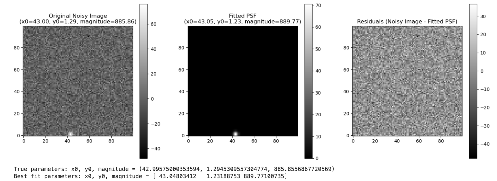
Fitted on subtracted data:
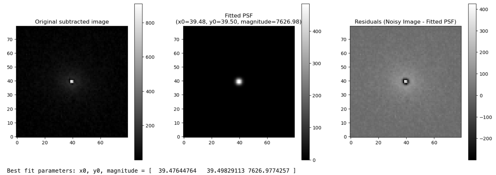
True max for subtracted img: 910.8002898616148
This is an analytical way to model the point source. Why not just using psf from Roman?
2024-09-08
Tutorial with SolidWorks

2024-08-27
CMB notebook:
#notes
Atacama Cosmology Telescope (ACT) and the South Pole Telescope (SPT): arc minute resolution
The mapmaking algorithms are not described here but represent a very interesting big data challenge as they require cleaning time streams by filtering, identifying transient events, and ultimately compressing ~Tb of data down to maps that are typically 100 Mb or less.
? clusters of galaxies which show up as darkened point sources:
Galaxies, or more specifically clusters of galaxies, show up as darkened point sources in CMB maps primarily due to the Sunyaev-Zel'dovich (SZ) effect.
The SZ effect occurs when the CMB radiation passes through a cluster of galaxies. The hot, ionized gas in these clusters interacts with the CMB photons, scattering them and slightly increasing their energy. This interaction causes a distortion in the CMB spectrum, leading to a decrease in the intensity (or temperature) of the CMB at certain frequencies, particularly in the range observed by telescopes like the South Pole Telescope (SPT) and the Atacama Cosmology Telescope (ACT).
In CMB maps, this decrease in intensity due to the SZ effect makes the clusters of galaxies appear as "darkened" spots. These spots are not truly dark but are relatively less bright compared to the surrounding CMB due to this scattering effect. The SZ effect provides a powerful tool for detecting and studying galaxy clusters, as the distortion it causes in the CMB is independent of the redshift of the cluster, allowing astronomers to detect clusters at a wide range of distances.
While the current instruments (ACTPol and SPTPol) have multiple frequencies and polarization sensitivity, for simplicity we consider only a single frequency (150 GHz) and only temperature.
multiple frequencies and polarization sensitivity?
show the basics of monty carlo analysis of both the angular power spectrum and matched filter techniques for studying Sunyaev-Zeldovich (SZ) effect.
-
Angular Power Spectrum: The angular power spectrum describes how the temperature fluctuations in the CMB vary with scale (or angular size on the sky). Monte Carlo simulations can be used to generate many random realizations of these temperature fluctuations based on theoretical models. By averaging the results, researchers can compare simulated data with observed data to understand the underlying physical processes and refine their models.
-
Matched Filter Techniques:
In the context of the paragraph you provided, matched filter techniques are used to study the Sunyaev-Zel'dovich (SZ) effect in Cosmic Microwave Background (CMB) data. Here’s how they work:-
Template Creation: First, a template or model of the expected signal (in this case, the SZ effect caused by galaxy clusters) is created. This template represents the known shape or pattern of the signal that the researchers are trying to detect.
-
Filtering: The matched filter is then applied by "matching" the data with the template. This involves sliding the template across the data and, at each position, calculating how well the data matches the template. This process enhances the signal's presence in the data, making it stand out more clearly against the background noise.
-
Detection: The output of the matched filter is a new set of data where the signal, if present, is more prominent. Peaks in this output indicate locations where the signal closely matches the template, suggesting the presence of the desired signal (e.g., a galaxy cluster affecting the CMB via the SZ effect).
-
Stacking analysis and cross-correlation
-
Stacking analysis is a method used to improve the signal-to-noise ratio (SNR) of a signal that is too weak to be detected in individual observations. The basic idea is to "stack" or average multiple observations of the same type of signal to enhance the signal while averaging out the noise.
-
Cross-Correlation: Cross-correlation is often used to compare the positions of galaxy clusters detected in CMB data with those detected in optical surveys. A peak in the cross-correlation function could indicate a strong alignment, suggesting that the same galaxy clusters are being detected by both methods.
2024-08-26
First day of class!!!
2024-08-23
compare to previous one:
Accuracy: 0.3155017371755569
Precision: 0.9028770369249959
Recall: 0.3155017371755569
F1 Score: 0.4669643350738403
2/2 [] - 0s 69ms/step - loss: 2.6353 - accuracy: 0.0877
Test Loss: 2.6352860927581787
Test Accuracy: 0.08771929889917374
2/2 [] - 1s 71ms/step
2024-08-22
unfreeze the initial layers:
Test Loss: 2.432490825653076
Test Accuracy: 0.28070175647735596
freeze all
2/2 [==============================] - 0s 64ms/step - loss: 2.4321 - accuracy: 0.0877 Test Loss: 2.4320554733276367 Test Accuracy: 0.08771929889917374
Want to learn more physics/astro, other than just the techniques.
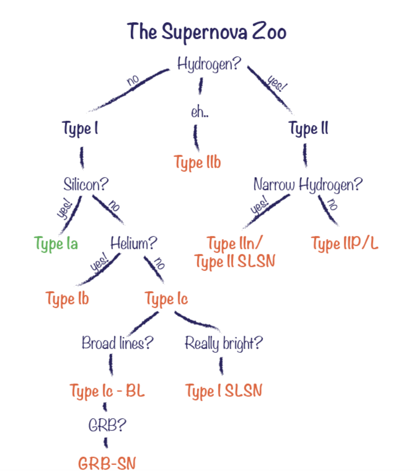
- "Classifying Supernovae"https://astrobites.org/2016/12/02/classifying-supernovae/
- Type Ia: we find them most often, and they can be used to study cosmology.
2024-08-21
Kostya Malanchev transfer model
ASTROMER, between different surveys:
https://ui.adsabs.harvard.edu/abs/2023A%26A...670A..54D/abstract
ATA: works on ELASsTiCC
https://ui.adsabs.harvard.edu/abs/2024arXiv240503078C/abstract
1 gal info:
Test Loss: 2.6169216632843018
Test Accuracy: 0.017543859779834747
2 gal info:
Test Loss: 2.635767698287964
Test Accuracy: 0.017543859779834747
2024 -08-20
preprocessed data under those two files are not the same (padded lightcurve size is different): processed_DES-SN5YR_DES and processed_for_training_DES-SN5YR_DES
processed_no_spec folder: padded for maximum step 264, and excluded no spec object
(568, 264, 4) light_curves_no_spec.shape
(568, 2)
Pretrained model on ELAsTiCC only has 1 host galaxy information (they only load 1 )
ELAsTiCC data from parquet file: in astropy table, with meta data for host gal information:
RA: 194.19433687574005
DEC: -16.671912911329965
MWEBV: 0.04543934017419815
MWEBV_ERR: 0.0022719670087099075
REDSHIFT_HELIO: 0.17915458977222443
REDSHIFT_HELIO_ERR: 0.18240000307559967
VPEC: 0.0
VPEC_ERR: 300.0
HOSTGAL_FLAG: 0
HOSTGAL_PHOTOZ: 0.17915458977222443
HOSTGAL_PHOTOZ_ERR: 0.18240000307559967
HOSTGAL_SPECZ: -9.0
HOSTGAL_SPECZ_ERR: -9.0
HOSTGAL_RA: 194.19388603872085
HOSTGAL_DEC: -16.671997552059448
HOSTGAL_SNSEP: 1.584566593170166
HOSTGAL_DDLR: 2.2270548343658447
HOSTGAL_CONFUSION: -99.0
HOSTGAL_LOGMASS: 10.462599754333496
HOSTGAL_LOGMASS_ERR: -9999.0
HOSTGAL_LOGSFR: -9999.0
HOSTGAL_LOGSFR_ERR: -9999.0
HOSTGAL_LOGsSFR: -9999.0
HOSTGAL_LOGsSFR_ERR: -9999.0
HOSTGAL_COLOR: -9999.0
HOSTGAL_COLOR_ERR: -9999.0
HOSTGAL_ELLIPTICITY: 0.16599999368190765
HOSTGAL_MAG_u: 22.44662857055664
HOSTGAL_MAG_g: 20.890161514282227
HOSTGAL_MAG_r: 19.744098663330078
HOSTGAL_MAG_i: 19.249099731445312
HOSTGAL_MAG_z: 18.987274169921875
HOSTGAL_MAG_Y: 18.772409439086914
HOSTGAL_MAGERR_u: 0.04701000079512596
HOSTGAL_MAGERR_g: 0.015930000692605972
HOSTGAL_MAGERR_r: 0.015960000455379486
HOSTGAL_MAGERR_i: 0.015799999237060547
HOSTGAL_MAGERR_z: 0.01576000079512596
HOSTGAL_MAGERR_Y: 0.015790000557899475
Transfer learning, how to deal with different target size?
Transfer target into a list: [0000001] list: AstroMCAD used it (and DES will run into error of too few objects. )
- AstroMCAD:
# Split normal data into train, validation, and test
X_train, X_temp, host_gal_train, host_gal_temp, y_train, y_temp = train_test_split(
	light_curves_no_spec, host_gals_no_spec, targets_no_spec, stratify=targets_no_spec, random_state=40, test_size=0.2
)

X_val, X_test, host_gal_val, host_gal_test, y_val, y_test = train_test_split(
	X_temp, host_gal_temp, y_temp, stratify=np.argmax(y_temp, axis=1), random_state=40, test_size=0.5
)
ValueError: The least populated class in y has only 1 member, which is too few. The minimum number of groups for any class cannot be less than 2.
- ELAsTiCC did not use this
# Train-validation-test split: 80% training, 10% validation, 10% test

X_train, X_test, host_gal_train, host_gal_test, y_train, y_test = train_test_split(x_data_norm, host_gal, y_data_norm, random_state = 40, test_size = 0.1)
X_train, X_val, host_gal_train, host_gal_val, y_train, y_val = train_test_split(X_train, host_gal_train, y_train, random_state = 40, test_size = 1/9)
[in progress] training for the new 2 galaxy info for ELAsTiCC
[in progress] trying to shrink current DES data to 1 d for galaxy info:
host_gal = sn_phot'REDSHIFT_FINAL', 'MWEBV'.values[0]
2024 -08-19
maximum timestep for lightcurve: max_timesteps (264 for DES)
Mismatch between pretrained and new model
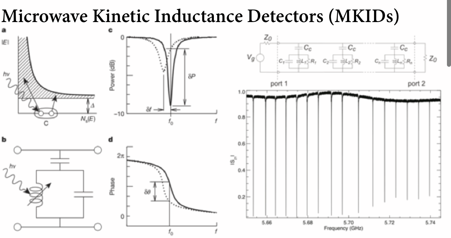
In a frequency-multiplexed system, a single readout system can monitor the signals from many MKIDs simultaneously by measuring the response of the system across a range of frequencies. Each MKID's signal will appear as a distinct peak at its specific resonance frequency. The readout electronics can then separate and process these signals based on their frequency.
Resources:
CMB: The McMahon Cosmology Lab - CMB Summer School
Modeling instrumentational noise: CMBAnalysis_SummerSchool/CMB_School_Part_03.ipynb at master · jeffmcm1977/CMBAnalysis_SummerSchool · GitHub
ZCU111 Evaluation Board manual: AMD Technical Information Portal
Readout software: primecam_readout/docs/docs_primecame_readout.ipynb at develop · TheJabur/primecam_readout · GitHub (from the canada team)
- One of the lessons learned from the first engineer- ing run of DemoCam[8] is that good magnetic shield- ing is essential for MKID operation. [web.physics.ucsb.edu/~bmazin/Papers/preprint/czakon_LTD13.pdf]
2024 -08-16
readout:
Fred Young Submillimeter Telescope (FYST)
Prime-Cam instrument
Kinetic inductance detectors (KIDs)
Microwave kinetic inductance detectors (MKIDs)
Radio Frequency System on a Chip (RFSoC)
2024 - 08-06
To do:
17. see if pre-trained model predicts our data
18. train our own model and predict
for task 1: Zero accuracy???
Accuracy: 0.0
Precision: 0.0
Recall: 0.0
F1 Score: 0.0
I probably should not use isolation model to predict labels, isolation forest is for anomaly detections.
Class weights?
2024 - 08-05
hyper-parameters to determine learning rate.
I'm losing a lot of data????
Try to debug!
AHHHHH yess, each SNID has multiple light curvesss! They're from different passband!
Model size issue...latent size needs to be fixed.
2024 -07-31
New results with correct matching.
Missing type 66
Try to plot and compare more results
Try to play with more data
2024-07-29
ZTF summer school:
Intro to ZTF Intro to ZTF
2024 -07-11
SNTYPE integer array:
array([101,   1,   0, 180,  80, 129,  29, 139,   4,  41,  23,  39,  66,
       141], dtype=int32)
Number of data too small:
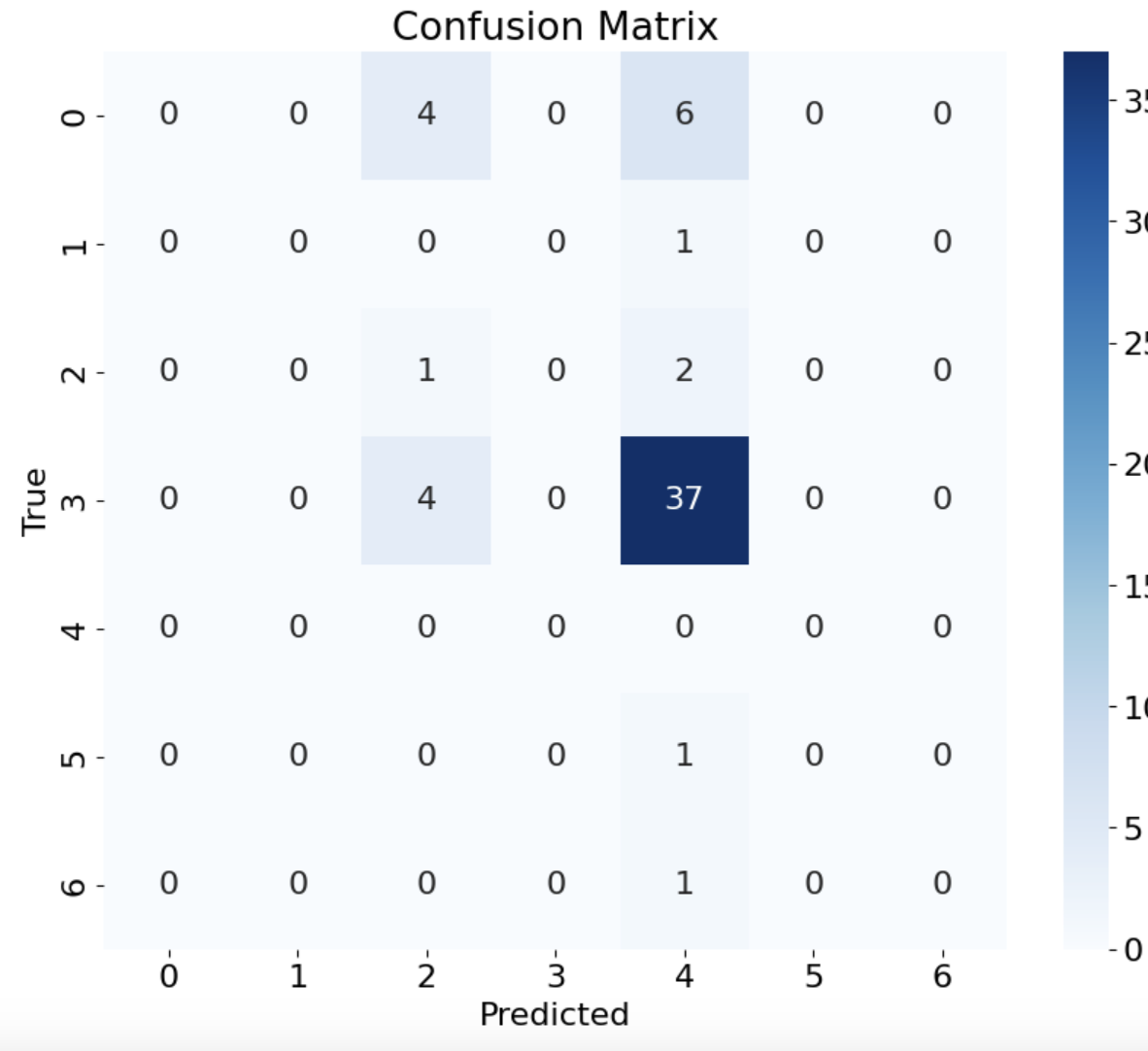
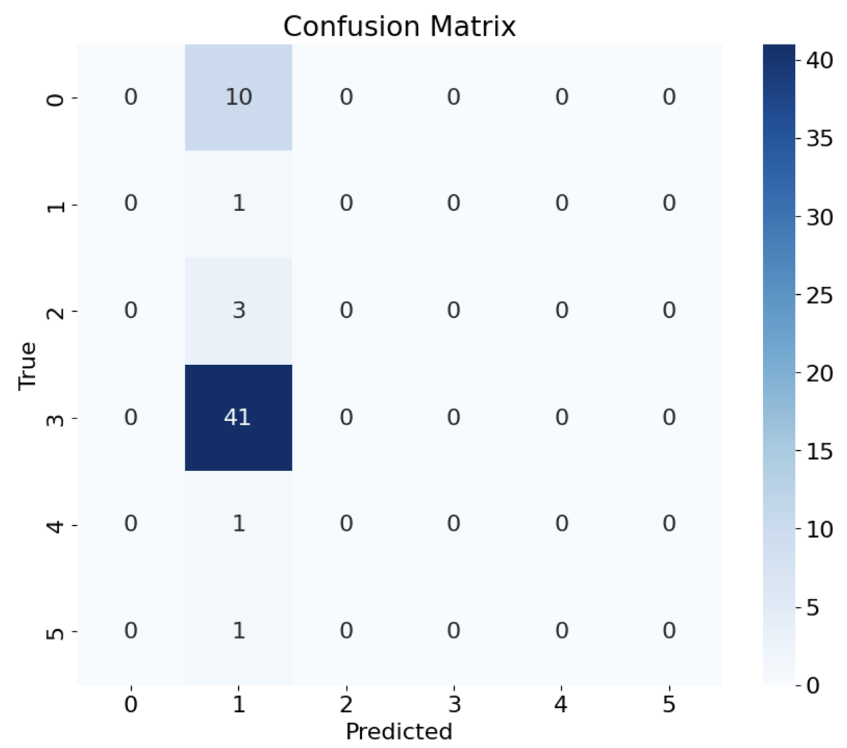
# Make Latex Table of counts for each training, validation, test, and all data

SNIa & 52 & 7 & 7 & 66 \\
\hline
IIL & 11 & 0 & 1 & 12 \\
\hline
SNII & 0 & 0 & 1 & 1 \\
\hline
Ibc & 1 & 0 & 0 & 1 \\
\hline
IIn & 1 & 0 & 0 & 1 \\
\hline
II & 1 & 0 & 0 & 1 \\
\hline
AGN & 16 & 4 & 2 & 22 \\
\hline
TDE & 1 & 0 & 0 & 1 \\
\hline
KNe & 0 & 0 & 4 & 4 \\
\hline
normal vs anomalous classes:
# Class names in the same order as the filenames
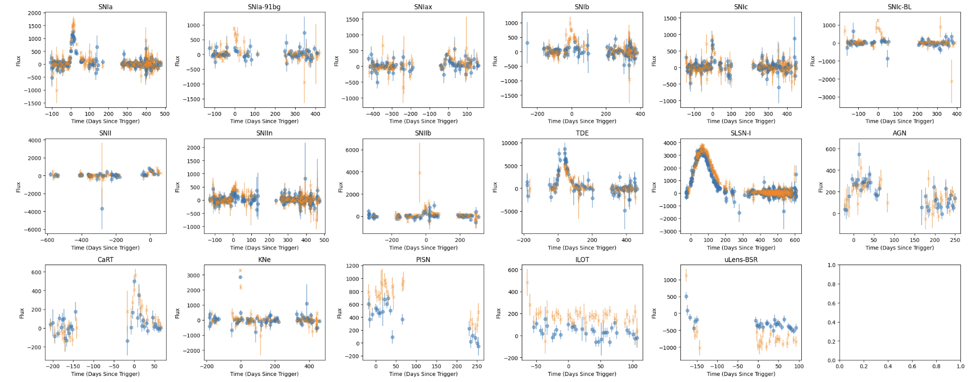
classes = ['SNIa', 'SNIa-91bg', 'SNIax', 'SNIb', 'SNIc', 'SNIc-BL', 'SNII', 'SNIIn', 'SNIIb', 'TDE', 'SLSN-I', 'AGN', 'CaRT', 'KNe', 'PISN', 'ILOT', 'uLens-BSR']
# Map class names to file names
class_to_file = dict(zip(classes, file_names)) # Dictionary from filename to the classname
# Define Anomalous Classes as the last 5 classes, and common classes as the first 12 classes
anom_classes = classes[-5:]
non_anom_classes = classes[:-5]
Different class lc looks like:
Count number of light curves for each class:
SNTYPE 0: 8133 light curves
SNTYPE 1: 66 light curves
SNTYPE 101: 22 light curves
SNTYPE 29: 12 light curves
SNTYPE 129: 4 light curves
SNTYPE 80: 4 light curves
SNTYPE 180: 1 light curves
SNTYPE 139: 1 light curves
SNTYPE 4: 1 light curves
SNTYPE 41: 1 light curves
SNTYPE 23: 1 light curves
SNTYPE 39: 1 light curves
SNTYPE 66: 1 light curves
SNTYPE 141: 1 light curves
SNTYPE Unknown: 8133 light curves
SNTYPE SNIa: 66 light curves
SNTYPE AGN: 22 light curves
SNTYPE IIL: 12 light curves
SNTYPE KNe: 4 light curves
SNTYPE Unclear: 4 light curves
SNTYPE Other Transients: 1 light curves
SNTYPE TDE: 1 light curves
SNTYPE SNII: 1 light curves
SNTYPE Ibc: 1 light curves
SNTYPE IIn: 1 light curves
SNTYPE II: 1 light curves
SNTYPE specific type: 1 light curves
SNTYPE Variable Star: 1 light curves
random mapping from integer to name that I use:
# Mapping of SNTYPE codes to their descriptions
sntype_mapping = {
    1: "SNIa",
    2: "SNIb",
    3: "SNIc",
    4: "SNII",
    20: "General Supernova",
    21: "General Supernova",
    101: "AGN",
    120: "AGN",
    129: "KNe",
    139: "TDE",
    141: "Variable Star",
    180: "Other Transients",
    80: "Unclear", #"Supernova with Spectral Classification but Unclear Type",
    0: "Unknown",
    29: "IIL",
    41: "Ibc",
    23: "IIn",
    39: "II", #(unspecified subtype)",
    66: "specific type"
}
ZTF summer school!!
ZTF Summer School | AI in Astronomy 2024
2024-07-10
AGN rate model
Model config file for AGN, to check for rate model:
qcheng@perlmutter:login11:/global/cfs/cdirs/lsst/groups/TD/SN/SNANA/SURVEYS/LSST/ROOT/ELASTICC/model_config
vim SIMGEN_INCLUDE_CLAGN.INPUT
NGENTOT_LC: 175000
DNDZ: POWERLAW 1.0E-3 0.0
GENRANGE_REDSHIFT: 0.1 2.9
From Rick: DN/DZ is actually R(z)
DNDZ is a volumetric rate vs redshift . Current AGN rate is constant volumetric rate and I don’t know conversion to NGENTOT. Pick a(1+z)^b model and set a to anything and b=0 and sim code will compute NGEN for a= volumetric rate
2024-07-08
Pretrained model from AstroMCAD:
github: 9 latent features
pip install version 1.2: 100 features.
2024-07-03
Meeting with Rick: Rate model:
For the extra-galactic models, model developer provides their rate model, which is usually related to redshift. We can discuss it with each author. For galactic models, it’s related to the coordinate and galactic plane, and we usually don’t have a good understanding of the rate model, but we can use the reference from the PLAsTiCC paper.
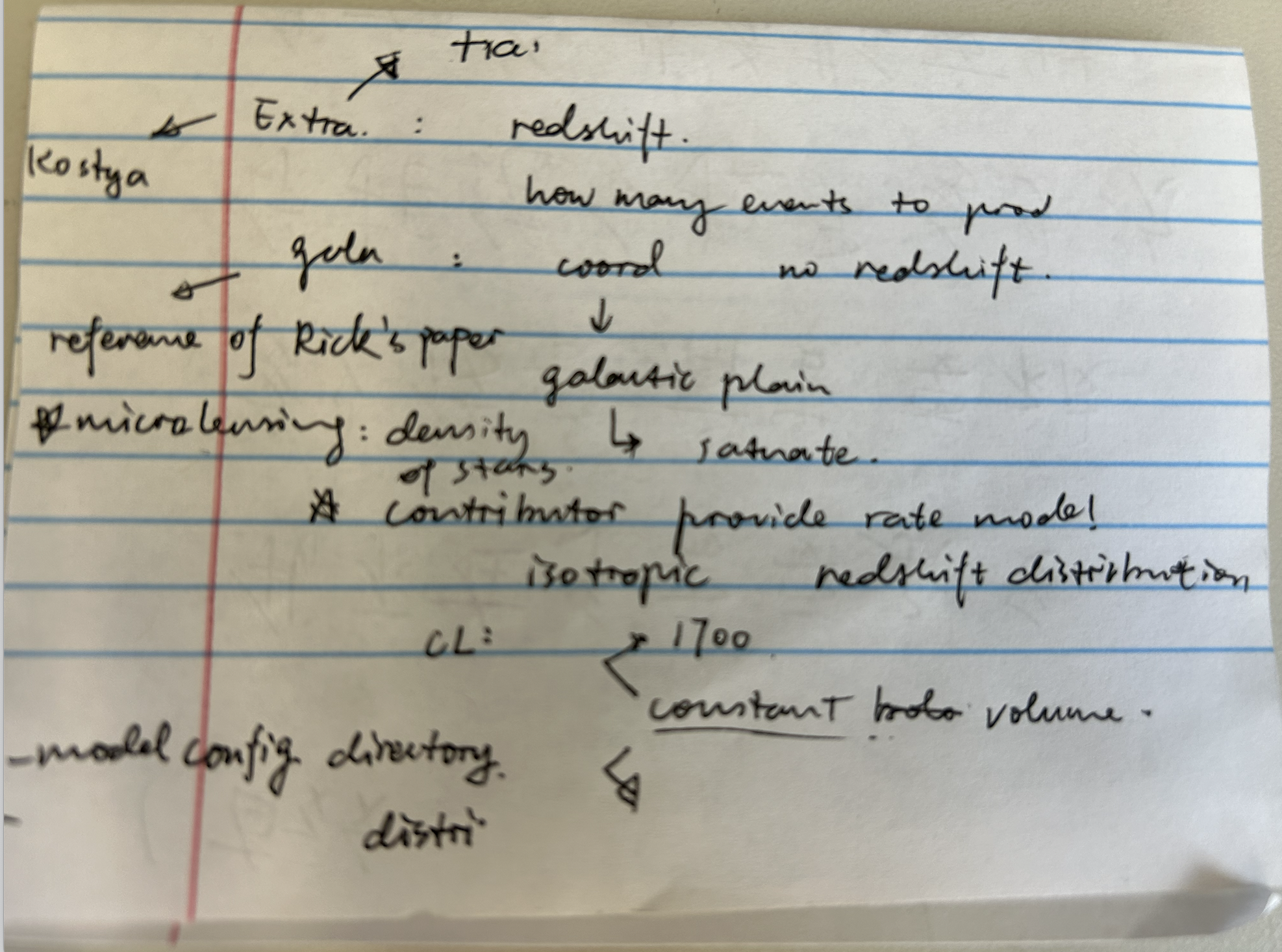
Mac address: internet port for each device
2024-06-23
Task:
process log
Target SN:
20148117 10.1320933873459 -44.99021376377029 62675.527
snid, ra, dec
Copy fits file to local computer, to open in DS9:
For SN peak:
scp [email protected]:/cwork/mat90/RomanDESC_sims_2024/RomanTDS/images/simple_model/Y106/47868/Roman_TDS_simple_model_Y106_47868_18.fits.gz Documents/2_Research.nosync/ngmix/
For galaxy:
scp [email protected]:/cwork/mat90/RomanDESC_sims_2024/RomanTDS/images/simple_model/Y106/52118/Roman_TDS_simple_model_Y106_52118_18.fits.gz Documents/2_Research.nosync/ngmix/
Cannot extract .gz inside Mac - Error identifying a writable temporary folder
❌sudo rm -rf /var/folders/*
The /private/var folder path is on the System read-only filesystem and you do not have permission to write (what you are really doing with a /bin/mv command) there. You might have been able to pull this off on an older (e.g. Mojave) version of macOS where the System partition was not protected, but with Catalina and later, you have no access privilege, even with Full Disk Access.
✅ unzip it somewhere else
Align images
Use reproject package! Fixed!!!!! Eventually!!!
# Reproject the entire SN image to the galaxy image's WCS
img_SN_reprojected, footprint = reproject_interp((img_SN, wcs_SN), wcs_galaxy, shape_out=img_galaxy.shape)

# Define the cutout position and size
position = SkyCoord(ra=10.1320933873459*u.deg, dec=-44.99021376377029*u.deg)
size = (100, 100)  # size in pixels

# Create cutouts from the reprojected images
cutout_galaxy = Cutout2D(img_galaxy, position, size, wcs=wcs_galaxy)
cutout_SN_reprojected = Cutout2D(img_SN_reprojected, position, size, wcs=wcs_galaxy)
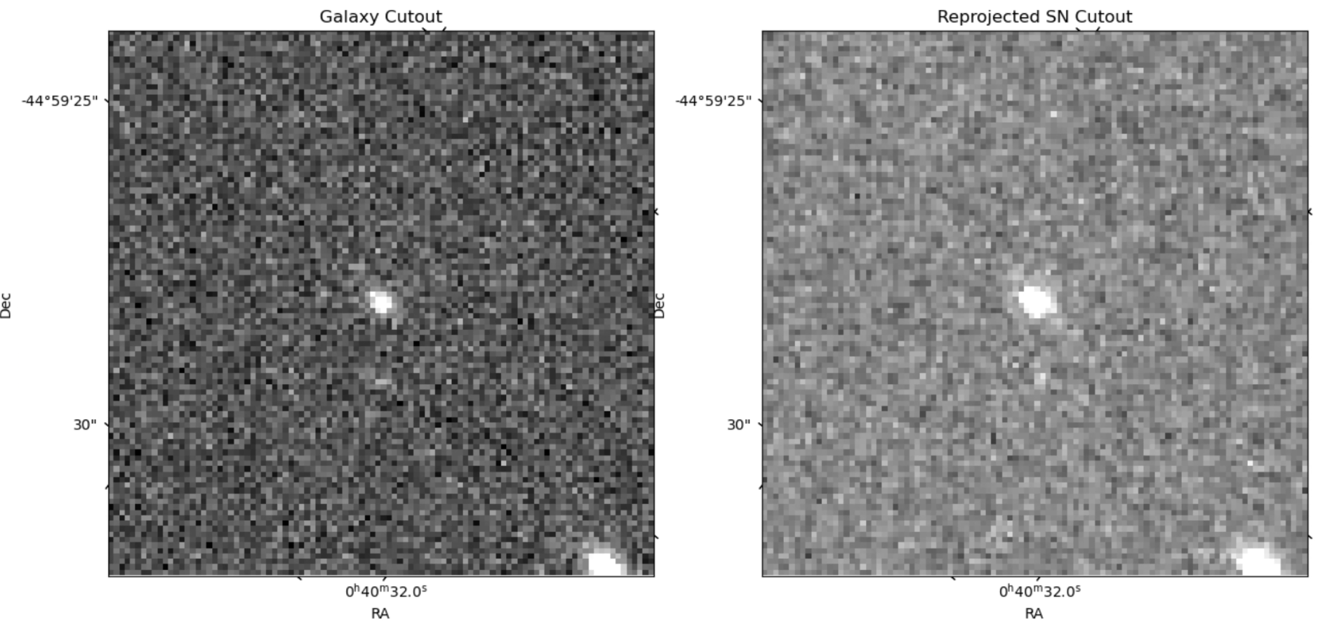
There are many undocumented struggling before this time point... But it's too painful to recall...
2024-03-19
#superphot
Issue:
Installation of superphot: Won't be able to build confluent_kafka
The problem with M1 is that Homebrew is installed in a different location and so these variables need to be added to the environment by including these lines in your .zshrc file
C_INCLUDE_PATH=/opt/homebrew/Cellar/librdkafka/1.8.2/include LIBRARY_PATH=/opt/homebrew/Cellar/librdkafka/1.8.2/lib pip install confluent_kafka
2024-03-20
Issue: Macos after install antares_client The kernel for appears to have died. It will restart automatically.
Firt solve around: Move code to .py file, and get more specific debugging prompt.
Error #15: Initializing libiomp5.dylib, but found libiomp5.dylib already initialized OMP: Hint: This means that multiple copies of the OpenMP runtime have been linked into the program. That is dangerous, since it can degrade performance or cause incorrect results. The best thing to do is to ensure that only a single OpenMP runtime is linked into the process, e.g. by avoiding static linking of the OpenMP runtime in any library. As an unsafe, unsupported, undocumented workaround you can set the environment variable KMP_DUPLICATE_LIB_OK=TRUE to allow the program to continue to execute, but that may cause crashes or silently produce incorrect results. For more information, please see [http://www.intel.com/software/products/support/](http://www.intel.com/software/products/support/).
Found solution online: python - Error #15: Initializing libiomp5.dylib, but found libiomp5.dylib already initialized - Stack Overflow
Solution to Error 15 Initializing libiomp5dylib, but found libiomp5 dylib already initialized
Issue: jax package not working
Solution: script written with old version of jax, where we need to import jax.config, but newer version of jax does not have jax.config. Downgrade.
2024-03-21
Issue:
In the tutorial, where it uses different sampler methods of "dynesty", "NUTS”, and “svi” to fit light-curves, I found “NUTS” model does not work. When we fit with “NUTS” sampler, the result is same as “svi” sampler, which can be told by the saved file name, sampling method attribute after the fit, and the output data/figure. I think they are not supposed to be the same. I checked out the source code but couldn't find a clue.
Already sent email to ask
Issue 2:
cannot import name 'adjust_log_dists' from 'superphot_plus.utils'
No such method in this file
Tired to run classifier.py:
No module named 'superphot_plus.file_paths'
No such file in the module.
2024-04-04
Try to do:
run astromcad
model galaxy from different model type
conda install pip to use local pip
Anomally detection:
Find the source code of the installed package:
import astromcad
print(astromcad.__file__)
Pip installed astromcad:
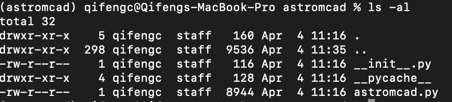
Missing 'pretrained' file
added to the package to the source code by hand (need absolute path)
AttributeError: Can't get attribute 'Custom' on <module '__main__' (built-in)>
python - Unable to load files using pickle and multiple modules - Stack Overflow
Need to import Custom explicitly in test.py file, where we run Detect.init()
ModuleNotFoundError: No module named 'keras.src.saving.pickle_utils'
Downgrading to TF==2.9
ERROR: Could not find a version that satisfies the requirement tensorflow==2.9 (from versions: 2.13.0rc0, 2.13.0rc1, 2.13.0rc2, 2.13.0, 2.13.1, 2.14.0rc0, 2.14.0rc1, 2.14.0, 2.14.1, 2.15.0rc0, 2.15.0rc1, 2.15.0, 2.15.1, 2.16.0rc0, 2.16.1)

ERROR: No matching distribution found for tensorflow==2.9
Need to downgrade python as well.
Downgraded to python3.8
AttributeError: 'Adam' object has no attribute 'build'
An issue with M1/M2: need later version of tensorflow. Or tensorlow-nightly
(astromcad) qifengc@Qifengs-MacBook-Pro astromcad % pip install tf-nightly

ERROR: Could not find a version that satisfies the requirement tf-nightly (from versions: none)

ERROR: No matching distribution found for tf-nightly
Stuck.... Let's do it tomorrow
2024-04-05
One way is to solve this adam issue:
Test tensorflow adam algorithm: works on my environment.
import tensorflow as tf

cifar = tf.keras.datasets.cifar100
(x_train, y_train), (x_test, y_test) = cifar.load_data()
model = tf.keras.applications.ResNet50(
    include_top=True,
    weights=None,
    input_shape=(32, 32, 3),
    classes=100,)

loss_fn = tf.keras.losses.SparseCategoricalCrossentropy(from_logits=False)
model.compile(optimizer="adam", loss=loss_fn, metrics=["accuracy"])
model.fit(x_train, y_train, epochs=5, batch_size=64)
Another way: try it in colab. Now error goes to later lines.
ValueError: Layer 'gru_cell' expected 3 variables, but received 0 variables during loading. Expected: ['gru/gru_cell/kernel:0', 'gru/gru_cell/recurrent_kernel:0', 'gru/gru_cell/bias:0']
Possible reason: Pretrained data version is different from keras version?
During the model loading process, the code attempts to deserialize the Keras model using deserialize_keras_object() function from the keras.saving.serialization_lib module.
Try another module (Custom):
Debugged source code:
NameError: name 'X_val' is not defined
Solved: the function defines x_val as input variable, but used X_val inside.
NameError: name 'class_weights' is not defined
Trouble shooting: the function is missing
between April and May:
The profiles that ngmix has:
Try bd according to Chien-hao's suggestion
2024-05-09
Try bd model:
2024-05-20
Sigma clipping
jupyter notebook connection
Jupyter notebook connection DCC
2024-05-23
setup code on cloud
building environment
import ngmix error:
Try to find if such file exisits:
find / -name "libstdc++.so*"
No root permission
Seems like only
Wroked!!!:
19. uninstall gcc: ngmix working, but jupyter broke:
(cosmo) qc59@dcc-login-05  **/hpc/group/cosmology/qc59 $** cat jupyter-notebook-9363580.log
ERROR: Unable to locate a modulefile for 'GCC/9.3.0'

FFTW 3.3.9-rhel8-intel

MPICH 3.2.1

GSL 2.6

install gcc-lib
(note on what have been uninstalled:)
(cosmo) qc59@dcc-login-05  **/hpc/group/cosmology/qc59 $** conda uninstall gcc

Channels:

 - defaults

 - conda-forge

Platform: linux-64

Collecting package metadata (repodata.json): done

Solving environment: done


## Package Plan ##


  environment location: /hpc/group/cosmology/qc59/miniconda3/envs/cosmo


  removed specs:

    - gcc


The following packages will be REMOVED:


  binutils_impl_linux-64-2.38-h2a08ee3_1

  gcc-12.1.0-h9ea6d83_10

  gcc_impl_linux-64-12.1.0-hea43390_17

  kernel-headers_linux-64-2.6.32-he073ed8_17

  libgcc-devel_linux-64-12.1.0-h1ec3361_17

  libsanitizer-12.1.0-ha89aaad_17

  sysroot_linux-64-2.12-he073ed8_17
- conda install libgcc: something looks weird on jupyter (it shows that jupyter lab not installed?) But it's working!!! I'm pretty satisfied
Total time used: 3 hours
ImportError: Unable to find a usable engine; tried using: 'pyarrow', 'fastparquet'.
A suitable version of pyarrow or fastparquet is required for parquet support.
Trying to import the above resulted in these errors:
- Missing optional dependency 'pyarrow'. pyarrow is required for parquet support. Use pip or conda to install pyarrow.
- Missing optional dependency 'fastparquet'. fastparquet is required for parquet support. Use pip or conda to install fastparquet.
Conda install won't work
Try conda uninstall and then pip install: won't work
Something wrong with jupyter notebook?
- checked on connection
- altered .sh file (commented out lines to source .barsch)
Reinstalled jupyter lab worked????
When running:
sn_ids = []
# These are the SNANA parquet files, which contain truth information for all transients injected
# into the RomanDESC sims. Collect all the transient IDs into a list:
path_to_sn_ids = '/cwork/mat90/RomanDESC_sims_2024/roman_rubin_cats_v1.1.2_faint/snana*.parquet'
file_list = glob(path_to_sn_ids)
for file in file_list:
    # Read the Parquet file
    df = pd.read_parquet(file)
    sn_ids.append(list(df['id'].values.flatten()))
AttributeError: module 'pyarrow.lib' has no attribute 'ListViewType'
Hi,
I found the issue. I had the3.0.0pyarrow version install via pip on my machine outside conda. I uninstalled it withpip uninstall pyarrowoutside conda env, and it worked. Maybe I don't understand conda, but why is my environment package installation overriding by an outside installation?
Thanks for leading to the solution.
To do:
- retrieve object filtered by min max mentioned by Lauren
- Trying modeling galaxy without a supernovae
Issues I have for this weeks work, and suggestions I got from the group meeting
- updated chi-square: doesn't seem right. Suggestions from the group: something relevant to Truth file?
- Images from Roman_sim may not be good for galaxy fitting, as the model may mistakenly fit SNe instead of the galaxy. I was thinking about using the image where SNe is dim, but we don't necessarily have those in the simulations. Suggestions from the group: 1. mask out SNe and model the galaxy. Or 2. Build a template for galaxy models with close-by images that does not have SNe.
2024-05-30
Model: fitvd
Explore another Anomaly detection package:
conda create --name <env_name> --file requirements.txt